Update: I added an
appendix at the bottom that provides the algorithm for the oil shock model. Per Bubba's suggestion, I am thinking of how to redisplay the URR plot to better guide the eye.
Following up on
my critique of Stuart Staniford's estimate of global cumulative endpoint production of oil (aka the URR estimate), I found enough additional misinformation or plain mistakes in SS's model to refine my macro peak oil model (
1,
2) further.
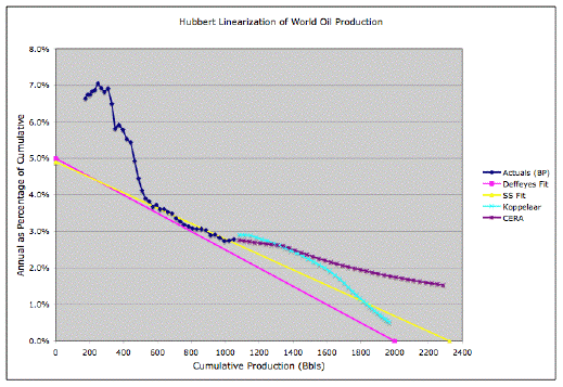
The mistake that Staniford made in applying the logistics model to BP's data came from the wrong initial (pre-1965) cumulative production. Look at the following plot from TOD and you see a telling "cusp" at the top of the curve:

That cusp disappears when one applies the right initial cumulative data; Staniford added about 100 Billion Barrels (BBls) too much to this data. This becomes obvious when you notice that his cumulative as of 2004 sits at about 1050 BBls -- 10% over the generally accepted value of 952 BBls from the
USGS.
This time I downloaded the data from BP's
World Energy 2005 page and tried to make a more decent try at a model fit. Based on comments at
The Oil Drum, two issues that I consider very important, (a) using historical data and (b) using realistic yet simple models, apparently tends to rub some people the wrong way. I think I have good arguments covering these concerns.
For some reason, the use of historical data causes certain oil watchers to scoff at us "backward" thinkers; they don't realize that we can learn a lot, both in a Bayesian sense and avoiding repeating the same mistakes over and over again (how shocking). Otherwise, I can only buy the argument up to a point; for example, until we hit the peak, we can't with 100% certainty predict the peak. Having a real inflection point or an obvious concavity does wonders for this class of analytical model.
I also find the simplicity of the model important -- something that Staniford agrees with. Unfortunately, he simplifies to such an extent, by using the Logistics curve, that he only has a single parameter to adjust. I find that much like having to make a prediction given only the
mean of some data set. I would at least like to have a couple of parameters, say the mean and
variance, to improve my chances. Here, Staniford throws away valuable information that has a good physical basis to achieve a simple empirical fit. I side with a good physical model that will give good intuition and insight to the problem at hand.
With that in mind I used my convolution-based Macro Peak Oil model to fit the BP data along with the USGS cumulative value of 952 BBls. The following uses a symmetric Triangular Discovery
1 curve starting in 1944 with a width of 87 years and normalized to an URR value of 2400 BBls.

The early years (pre 1970) of my model feature an oil extraction rate of 6% of total content per year. For an exponential drop-off, this gives a
1/e point of approximately 16 years.

I add three shocks in the years 1973-1974, 1979-1980, and 1991-1992, whereby the oil extraction rate changed dramatically. Because of the stationary properties of the Markov model, I can simply adjust the rates of the normalized exponential term in the middle of the convolution without violating the stochastic nature of oil extraction over time. The shocks tend to momentarily suppress and flatten the production/consumption rate. (As a technical aside, the suppressive dip in the output comes about mathematically from the exponential normalization)
The three shocks correspond to the OPEC embargo, Iranian crises coupled with a deep recession, and the first Gulf war.
| Year | Extraction Rate | %change |
|---|
| pre-1973 | 6% | N/A |
| 1973-1974 | 4.5% | -25% |
| 1979-1980 | 2.7% | -40% |
| 1991-1992 | 2.4% | -11% |
No doubt we will get more shocks in the future. The crucial finding in my mind: the shocks serve to delay
significantly the onset of peak oil. Before the 70's, we used oil as if it came out of the tap; we have since made significant corrections in the extraction rate and our more conservative use of oil. We will likely get a shock fairly soon -- this will not invalidate the model results and it will not disprove the peak oil hypothesis. It simply will serve to delay the peak a bit more. I really believe (and the model shows) that we would have hit a peak several years ago without these shocks in place.
Recession is good? How about that for back-handed insight?The final URR fit looks like the following curve. Of course the asymptote hits 2400 BBls because of the triangular distribution I started with. I mainly want to demonstrate how the annoying cusp disappears when plotted correctly.

1 I chose the triangular curve because of the proliferation of the following type of data.

Note that I use the term "discovery" a bit loosely; in my mind it actually indicates when pumping activity actually started on the previously discovered reserves.
APPENDIXThis code compiles with the GCC
gnatmake compiler provided with most recent vintages of Linux (or available for Windows
here). To build, save as file "shock_model.adb", then
gnatmake shock_model to make the executable. Spreadsheets like the CSV-format: "year", "BBls/day", "cumulative BBls"
with Text_IO;
with Ada.Numerics.Elementary_Functions;

procedure Shock_Model is

  subtype Years is Natural range 1944 .. Natural'Last;

  type Shock is record
    Year : Years; -- Year of shock
    Rate : Float; -- Prod. or depletion rate (fraction / year)
  end record;
  type Shocks is array (Years range <>) of Shock;

  Width  : constant := 87;      -- Triangle window
  Volume : constant := 2400.0;  -- In BBls

  S : constant Shocks :=
   ((Years'First, 0.06), -- Starting Year
    (1974, 0.048), -- OPEC
    (1980, 0.035), -- Iran +
    (1983, 0.029), -- Recession
    (1991, 0.026), -- Gulf I
    (2150, 0.0)); -- Ending Year

  --##### You don't have to look beyond this point unless you
  --##### want to mess with the algorithm or output.

  -- General purpose array of floats indexed by year
  type Flt is array (Natural range <>) of Float;

  -- Safe array get function, truncates values out of range
  function Get (Arr : Flt; I : Integer) return Float is
  begin
    if I in Arr'Range then
      return Arr (I);
    else
      return 0.0;
    end if;
  end Get;

  -- Takes 2 arrays and returns the convolution array
  function Convolve (A, B : in Flt) return Flt is
    Total : constant Natural := A'Length + B'Length;
    C     : Flt (0 .. Total);
    V     : Float;
  begin
    for J in  0 .. Total loop
      V := 0.0;
      for I in  0 .. J loop
        V := V + Get (A, I) * Get (B, J - I);
      end loop;
      C (J) := V;
    end loop;
    return C;
  end Convolve;

  -- Creates a symmetric window, truncated left by Start
  -- The prior accumulated data is provided by Impulse
  function Triangle_Window
   (Width   : in Natural;
    Start   : in Natural := 0;
    Impulse : Float      := 0.0)
    return    Flt
  is
    R      : Flt (0 .. Width - 1 - Start);
    Half   : constant Natural := Width / 2;
    Offset : Natural;
  begin
    for I in  R'Range loop
      Offset := I + Start;
      if Offset < Half then
        R (I) := Float (Offset) / Float (Half);
      else
        R (I) := Float (Width - Offset) / Float (Half);
      end if;
    end loop;
    R (0) := R (0) + Impulse;
    return R;
  end Triangle_Window;

  -- An exponential array populated to length
  function Exponential (Length : in Natural;
                        Alpha : in Float) return Flt is
    use Ada.Numerics.Elementary_Functions;
    R : Flt (0 .. Length - 1);
  begin
    for I in  0 .. Length - 1 loop
      R (I) := Alpha * Exp (-Alpha * Float (I));
    end loop;
    return R;
  end Exponential;

  -- The summed difference between two arrays up to Width
  -- This is used to renormalize when an Alpha rate changes
  function Leftover (A, B : in Flt;
                     Width : in Natural) return Float is
    V1 : Float := 0.0;
    V2 : Float := 0.0;
  begin
    for J in  0 .. Width - 1 loop
      V1 := V1 + Get (A, J);
      V2 := V2 + Get (B, J);
    end loop;
    V1 := V1 + 0.5 * Get (A, Width);
    V2 := V2 + 0.5 * Get (B, Width);
    return (V1 - V2);
  end Leftover;

  -- Recursive formula to re-convolute on successive rate shocks
  -- Returns production curve in array
  function Gen
   (S     : in Shocks;   -- Input stimulus
    Left  : in Float;    -- Pre-history reserve level
    Curve : in Flt;      -- The starting curve
    TS    : in Natural)  -- TimeSpan of results
    return  Flt
  is
  begin
    if S'Length = 1 then  -- returns on completion
      return Curve;
    else
      declare
        W1 : constant Natural := S (S'First).Year - Years'First;
        W2 : constant Natural := S (S'First + 1).Year - Years'First;
        T  : constant Flt     := Triangle_Window (Width, W1, Left);
        R  : constant Flt     :=
          Convolve (T, Exponential (TS, S (S'First).Rate));
      begin
        return Gen
                (S     => S (S'First + 1 .. S'Last),
                 Left  => Leftover (T, R, W2 - W1),
                 Curve => Curve & R (1 .. W2 - W1),
                 TS    => TS);
      end;
    end if;
  end Gen;

  Time_Span : Natural      := S (S'Last).Year - S (S'First).Year;
  R         : constant Flt := Gen (S, 0.0, (0 => 0.0), Time_Span);

  Total : Float          := 0.0;
  K     : constant Float := Volume / Float (Width) * 2.0;
begin
  for I in  R'Range loop
    Total := Total + K * R (I);
    Text_IO.Put_Line
     (Integer (Years'First + I)'Img & "," &     -- Year
      Float'Image (K * R (I) / 365.0) & "," &   -- Per Day
      Float'Image (Total));
  end loop;
end Shock_Model;
As a check, the red curve displays the output of the above code. The yellow curve shows what would have happened without the oil shocks. Through the roof, baby.


 Get yourself a good programmable current source with a storage oscilloscope measuring the shunted current through the resistor, and you can make your own Analog Peak Oil Simulation!1
 The actor who played Butch (the "bully") on the
 What does the right wing media think of data like this? Well, as I write this, I listen to Matt Drudge pontificate on his weekly radio show on "real" hurricane data as part of his "Global Warming Emergency Declared!" themed discussion. He goes on to list various Cat 4 and Cat 5 storms that have occurred over the last century, strangely interspersed with condemnations of celebrities like Barbra Streisand who show an interest in current events. Never mind the fact that the exception does not prove the rule in statistics, but bringing in celebs as some kind of elitism metric shows what kind of rejected outlier Drudge himself has become.
  OK, make the call to the deceased
  On Air America's
  Think about it. The TCS gang works themselves into a tizzy over a select group of politicians' opposition to LNG terminals, all the while, and as a matter of principle, ignoring every other facet of our energy predicament. Granted the democrats and moderate republicans have taken a populist view to price increases (i.e. gouging), but it sure beats the obvious corporate cheerleading and BushCo-styled greedy cronyism that TCS forever practices.
 Please, someone sign up James Glassman to play the whiny, insecure, almost paranoid character of


 Update: AAR's EcoTalk will have climate chaos


