Geostatistics a fraud?

The academic field of "economic geology" seems to cover the exploitation of resources rather than stewardship of the resources [TOD link]. If somebody in this research area had actually wanted to or had the charter to, they could have done an impartial study of resource depletion based on some rather simple models. The fact that a branch of this field is called "geostatistics" makes one think that somebody must be doing original research. But looking at the Wiki entry for geostatistics and the Wiki entry for the "father" of geostatistics, Matheron, you find lots of controversy.

And then, following the links, you also find that a web-site exists with the URL http://www.geostatscam.com, subtitled "Geostatistics: From human error to scientific fraud" . The engineer who runs the site, Jan Merks, makes the strong claims that the specialty of geostatistics consists of "voodoo statistics" and "scientific fraud". Granted, it looks like this criticism resides mainly in the context of mineral mining and perhaps petroleum extraction is not really a part of this field, but it makes you wonder what exactly constitutes research in geostatistics. A sample of Merks' charges:

Degrees of freedom fighters amongst professional engineers and geoscientists are addicted to Matheron's junk science of geostatistics. Hardcore krigers and cocksure smoothers turned mineral exploration into a game of chance with the stakes of mining investors.

From what I understand about the technique known as "kriging", it seems to provide a way to interpolate potential mineral deposits from sampled spatial measurements in surrounding areas. The criticism leveled on this technique rests on the observation that geostatisticians never want to provide a sound estimate of the variance of their interpolation. According to Merks, they at best create a phony variance to justify their estimate. If this is indeed so, I would agree that we should seriously look into what weird interpolations geostatistics considers as science.

As a counter-example, in all the models I use for oil depletion, I always use a huge variance consistent with the Maximum Entropy Principle. An assumed variance such as this maximizes the disorder, and provides the best estimate for reasoning under uncertainty. In other words, if you don't know the variance, you have too assume the worst case. The bad kriging estimates seem to basically say that if point A has X mineral grade and point B has Y mineral grade, then point C halfway between A and B has (X+Y)/2 mineral grade. From what I understand, unless you have a real spatial correlation between the points (which apparently no one verifies) no way can you do a naive interpolation like this. I have written papers on spatial correlation and always start by looking for the presence or lack of statistical independence between separated points.

So if geostatistics treats probability and statistics like a cook interpolates half-a-cup of bleached flour, the field has serious problems. It brings up the rather obvious question, why do they teach this? Do they realize the sad fact that exploration works at best as a pure crap-shoot and you might as well get the fresh eager graduates out in the field with nothing more than a pair of dice? Are the rockhead geologists that jaded?

H G Wells predicted that statistical thinking would become as important as the ability to read and write. Would Wells have embraced the nouveau pseudo science of interpolation without justification with the same unbridled passion as the world's mining industry did? [from Merks website]

Kernel of Logistic for Dispersive Discovery

The derivation of the dispersive discovery curve builds from a premise that individual discovery trajectories act on an ensemble of subvolumes within a larger volume (for example, the earth). Although the average rate of these arcs show an exponential acceleration over time, the individual rates get dispersed according to the Maximum Entropy Principle. The subvolumes also show an exponential PDF of sizes corresponding to the disorder expected in the geological search sizes of varying oil-bearing regions around the earth. Once the cumulative search in a subvolume completes, it reaches an asymptotic value proportional to the amount of oil in that region.

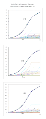
The following figure shows several Monte Carlo (MC) simulations of the build-up of the logistic Dispersive Discovery profile. This set of charts features only 100 sample traces accumulated per solid black line, yet the characteristic S-shape shows up clearly. The dashed curve behind the MC cumulative represents the logistic sigmoid function corresponding to theory.

In each of these cases, a gradual build-up of the individually colored profiles lead to nearly identical characteristic cumulative curves (save for counting noise).

I used a spreadsheet for this simulation as the MC algorithm reduces to a short algorithm. In the following formula, two exponential random variates sit in cells D$1 (growth dispersion) and D$2 (subvolume dispersion). An incremental time runs along column $A. The SIGN function truncates the individual cumulatives to truncate when the search reaches the subvolume limit. The term $A$1 represents the scaling term for the characteristic dispersion velocity spread. The last term acts like an integrator for $D$4 from the previous time step value D3.

+D$1*(SIGN(D$2-(D$1*$A4)/$A$1)+1)/2/$A$1+D3

If the time/$A series shows a linear growth in time, the summation of a series of these results in a hyperbolic asymptotic growth. If the time accelerates, we get the logistic form.

Each of the subvolume traces represent a discovery kernel function similar to a shocklet kernel. The physical realization of this becomes very intuitive, as prospecting for oil requires a complete survey of an entire subvolume, with the search accelerating over long periods of time as new technologies and tools become available. On the other hand, searches over very small regions may not have the aid of accelerated search and so the hyperbolic asymptotic growth results. This gives us the characteristic creaming curve in smaller basins. If you can understand when accelerating search applies and when linear search applies, it becomes very easy to predict what type of profile will occur in a region.

One thing I notice in the MC simulation is that the long term noise becomes greater as fewer discoveries contribute to the tail end of the curve. This may get reflected in the real statistics we will see as rather sparse fat-tail discoveries contribute to a long term decay.

A commenter at TOD recommended this visual as an aid to understanding how dispersion works.

Creep Failure

As a follow-up to the dispersive failure analysis I found a potential behavior that illustrates the early failure profile in a less abstract and perhaps more realistic manner.

Due to dispersion, a slow linear rate of growth in the breakdown process will lead to an early spike in the failure (or hazard) rate. This becomes the characteristic leading downward slope in the bathtub curve.

Figure 1: Linear into accelerating growth function

The enhanced early probability of failure arises purely through the spread in the failures through disorder mechanisms just as in the popcorn popping experiment. This in general leads to a bathtub shape with an analogy to the life-span of the human body (infant mortality, maturity, old age). For mechanical equipment, the shape in (b) provides a more realistic portrayal according to some.

Figure 1: Empirically observed bathtub curves
(a) electronics components (b) mechanical components

I earlier had abstracted away the velocity of the failure stimulus and integrity of the component to generate a parametric expression for the failure rate.

r(t) = dg(t)/dt / (tau + g(t))

In a real situation the velocity/integrity abstraction might occur as a stress/strain pairing particularly in a mechanical component.

We scale the integrity of the component as a physical dimension; it could be a formally defined measure such as strain, but we leave it as an abstract length for the sake of argument. The process acting on this abstraction becomes a velocity; again this could be a real force, such as the real measure of stress. [link]

In this case, a mechanism called creep can play a big role in determining the failure dynamics. Creep happens to a load under a constant stress condition over a period of time. This leads to a curve as shown below, which demonstrates a relatively quick rise in strain (i.e. deformation) before entering a linear regime and then an exponential as the final wear-out mechanism becomes too great.

Figure 3: Creep curve which physically realizes the growth function of Figure 1.

Although the stress/strain relationship can get quite complex, to first-order, we can compare the curve in Figure 3 to the general curve in Figure 1. The monotonic increase in the abstract growth term, g(t), remains the same in both cases, with both a linear and exponential regime noticeable in the middle (secondary) and late (tertiary) periods. The big difference lies in the early (primary) part of the curve, where due to elastic and plastic deformation (particularly in a viscoelastic material) the growth increases rapidly before settling into the linear regime. This fast "settling-in" regime intuitively provides a pathway to an earlier failure potential than a purely accumulating process would.

One can approximate the general trend in the primary part of the growth either by a rising damped exponential or by a parabolic/diffusive growth that rises with the n'th root of time. The following figure uses a combination of a square root and the exponential growth to model the creep growth:

g(t)= A*sqrt(kt) + B*(e^-ct -1)

Figure 4: Modeled creep growth rate

Applying this growth rate to the dispersive failure rate, g(t), we get the following bathtub curve.

Figure 5: Bathtub curve for growth rate exhibiting physical creep has a sharper initial failure rate fall-off due to earlier deformation.

Clearly, the early part of the curve becomes accentuated relative to the linear growth mechanism, and a more asymmetric v-shape results, characteristic of the mechanical failure mode of Figure 1(b).

References:

1. The physics of creep: creep and creep-resistant alloys, F. Nabarro, H. De Villiers, CRC Press,1995.

Verifying Dispersion in Human Mobility

Another article in Nature supports the model I put together for human mobility patterns
http://mobjectivist.blogspot.com/2009/10/scaling-laws-of-human-travel.html

My model seems to match the observed trends even more precisely and further reinforces the fundamental idea of entropic dispersion of travel velocities. Instead of using a paper money tracking system as in the previous Brockmann article, the authors (Gonzalez et al) used public cell-phone calling records -- this seems to perform more directly rather than the indirect mechanism of proxy records of bill tracking to monitor human mobility.

Given that money is carried by individuals, bank note dispersal is a proxy for human movement, suggesting that human trajectories are best modeled as a continuous time random walk with fat tailed displacements and waiting time distributions.
...
Contrary to bank notes, mobile phones are carried by the same individual during his/her daily routine, offering the best proxy to capture individual human trajectories.
...
Individuals display significant regularity, as they return to a few highly frequented locations, like home or work. This regularity does not apply to the bank notes: a bill always follows the trajectory of its current owner, i.e. dollar bills diffuse, but humans do not.

Even though the proxy records give the same general fat-tail trends, the essential problem with the bank note process remains the transaction process. The very likely possibility exists that a dollar bill exchanges hands among three unique individuals at a minimum between reporting instances, yet the cell-phone records an individual at more randomized and therefore less deterministic intervals.

So I don't expect the average rates of travel to necessarily agree between the two data-sets.

The following fit uses the same model as I used previously, with data sampled at 1 week intervals. Notice that the data fits the Maximum Entropy Dispersion (the green curve) even better than bill tracking at 10 day intervals.

dP/dr = beta*t/(beta*t+r)^2

The value of beta for this data set is 0.36 instead of 1 for the bill dispersion data set. I placed a cutoff on the dispersion by preventing a smearing into faster rates of 400 km/day and above, but this seems fairly reasonable as the model otherwise works over 5 orders of magnitude. It actually works so well that it detects a probability offset in the original data calibration; the probability PDF should sum to one over the entire interval yet the Gonzalez data exhibits a bias as it creeps up slightly over the normalized curve. This is real as their own heuristic function (when I took the time to plot it) also shows this bias.

Another figure that Gonzalez plots mines the data according to a different sampling process, yet the general trend remains.


Moreover, the researchers almost got the Maximum Entropy dispersion function right by doing a blind curve fit, but ultimately could not explain it. Instead of the predicted power-law exponent of -2, they use -1.75. Yet since they do not normalize their curve correctly with the beta parameter that a probability distribution requires, they think this value of -1.75 holds some significance. Instead the -1.75 power law is likely an erroneous fit and -2 works better -- while not violating Occam's law.

Entropy always wins out on these phenomena and it really tells us how (in the sense of having no additional information, i.e. a Jaynesian model of entropy) people will statistically use different forms of transportation. The smearing occurs over such a wide range because people will walk, bicycle, residentially drive, freeway drive, or take air transportation. The entropy of all these different velocities serves to generate the dispersion curve that we empirically observe. The fact that it takes such little effort to show this with a basic probability model truly demonstrates how universal the model remains. The bottom line is that a single parameter indicating an average value of dispersive velocity is able to map over several orders of magnitide; only a second-order correction having as much to do with the constrained physical breadth of the USA and how fast people can ultimately travel in a short period of time prevents a complete "single parameter" model fit.

Ultimately, what I find interesting is how the researchers in the field seem to flail about trying to explain the data with non-intuitive heuristics and obscure random walk models. Gonzalez at al have gotten tantalizingly close to coming up with a good interpretation, much closer than Brockmann in fact, yet they did not quite make the connection. If I could tell them, I would hint that their random walk is random but the randomness itself is not randomized. That explains so many phenomena yet they can't quite grasp it.

References:

1. Understanding individual human mobility patterns, Marta C. González, César A. Hidalgo & Albert-László Barabási, Nature 453, 779-782 (5 June 2008)

There is an Addendum (12 March 2009) associated with this document.

The Scaling Laws of Human Travel

I spotted a fairly recent-vintage paper on the statistics of human travel published in Nature magazine. This had the novelty of using the internet to collect indirect travel information by compiling the spread of money, via the bill tracking system http://www.whereisgeorge.com.

I can't argue the basic premise behind the approach. The authors, Brockmann, et all, assume that people disperse throughout a geographic region and make the claim that you can essentially track their motion (indirectly) by following the trajectory of the money they carry. They also make the correct interpretation that dispersion via random walk mechanisms plays a big role in the spread. That part seems quite reasonable. And the utility of understanding this phenomena holds great promise. For example, one can use it to understand the implications of reducing the travel overhead as we enter an energy-scarce era, as well as understanding the dynamics of pandemics. Yet, considering how important the concept is and the prestige of the journals that publish the work, they completely hose up the mathematics behind the phenomena. By that I mean they made the result horribly complex and opaque.

If they had used the correct formulation of dispersion, the agreements to their premise would have shown a very simple universality; yet they invoke some sophisticated notion of Levy flights and other esoteric models of stochastic mathematics to derive an overly complex result. Eventually they come up with a scaling law exponent which they affix with the value 0.59 and 1.05. They claim these odd numbers holds some notion of "universality" and claim that this results in some new form of "ambivalent" process. It seems a bit pretentious and I will use this post to derive some actual, much more practical, laws. For context, my own arguments use some of the same concepts that I have used for Dispersive Discovery of oil.

The statistics of what they want to model stems from sets of collected data from timestamped geographical locations. The figure below shows typical vector traces of travel across the USA.

Figure 1 : Typical bill travel traces due to Brockmann

The collected information appears very comprehensive and the fact that everyone uses money, attests to the fact that the approach should show little bias with minimal sample error. I don't have the data directly in my hands so some parts I may have misinterpreted, but so far so good.

We part company from that point. I don't really care to know the sophisticated random-walk model they use but it appears pretty much derived from the Scher-Montrose Continuous Time Random Walk (CTRW) model that I have looked at previously (see
http://mobjectivist.blogspot.com/2009/06/dispersive-transport.html and notice how that problem on a microscopic scale is similarly overly complicated)

Instead of overt formality, I would set up the mathematical premise straightforwardly. We have a dispersion of velocities described by a maximum entropy probability distribution function (PDF).

p(v) = alpha*e^-alpha*v

The PDF above describes a mean velocity with a standard variance equal to the mean. This places all moments as finite values and becomes an intuitive minimally biased estimate considering no further information is available. We next assume that the actual distance traveled happens over a period of time.

The authors first describe a PDF of money traversing a distance r in less than 4 days.

p(r | t less than 4 days) = probability that the bill traveled r distance in less than 4 days

This becomes very easy to solve (if we assume that the distance traveled is uniformly distributed across the interval -- another maximum entropy estimator for that constraint). So for any one time, the cumulative distance traveled at any one time is expressed by the following cumulative distribution function (CDF), with r scaled as a distance:

P(r,t) = e^-alpha*r/t

The term alpha has the units of time/distance. As we haven't considered the prospects of waiting time variation yet, this point provides a perfect place to add that to the mix. Intuitively, money does not constantly stay in motion, but instead may sit in a bank vault or a piggy bank for long periods of time. So we smear the term alpha again with a maximum entropy value.

p(alpha) = beta*e^-beta*alpha

But we still have to integrate this over all smeared values, with respect to P(r,t). This gives the equation

P(r,t) = beta/(beta + x/t)

To generate the final PDF set, we take the derivative of this equation with respect to time, t, to get back the temporal PDF, and with respect to r, to get the spatial PDF (ignoring any radial density effects) .

dP/dt = beta*r/(beta*t+r)^2
dP/dr = beta*t/(beta*t+r)^2

So we can generate a PDF for r for a specific value of T=4 days and then fit the curve to a value for beta. So beta becomes the average velocity/waiting time for a piece of paper money (the bank note the authors refer to) between the times it makes trips from place to place. This approach only differs from the use of dispersion for oil discovery in the fact that velocity shows a greater dispersion than it would otherwise; the fact that time acts as the dispersive parameter and this goes in the denominator of velocity=r/t, implies that the fat tails appear in both the spatial dimension and the temporal dimension.

Figure 2: Contour profile in spatial/temporal dimensions for
dispersion of money. High levels and hot colors are high probability.

To verify the model, the authors plot the results in two orthogonal dimensions. First against time:

P(t | r less than 20 kilometers) = The probability that a bill has traveled 20 km or less in a set time.

The constrained curve fits are shown below with beta set to 1 kilometer per day. The various sets of data refer to 3 classes of initial entry locations (metropolitan areas, intermediate cities, and small towns).

Figure 3a and 3b: Profiles of probability along two orthogonal axis.
The red lines are fits for dispersion with beta = 1.

The short-distance spatial curve has some interesting characteristics. From the original paper, a plot of normalized probabilities shows relative invariance of distance traveled with respect to time for short durations of less than 10 days.

Figure 4: Contour profile from Brockmann.

Time appears bottle-necked for around 10 days on the average. This is understandable as the waiting time between transactions can contain 5 distinct stages. As most of these transactions may take a day or two at the minimum, it is easy to conceive that the total delay is close to T=10 days between updates to the bill reporting web site. So this turns into a weighted hop invariant to time but scaled to reflect the average distance that the money would actually travel.

Figure 5: Latency at short time intervals has to go through 5 processing steps.
This is similar to what occurs in oil processing, see here.

If we plot our theory on a similar color scale, it looks like the 2-dimensional profile below. :

Figure 6: Contour plot of scaled probability values.
This shows good agreement with the Brockmann data in Figure 4.

Note that these look different than the first contour color scale in Figure 2 since the authors multiplied the probability values by r to maintain a similar dynamic range across all values. Otherwise the probability values would diminish at large r or t.

Figure 7: Alternate perspective of Figure 6. Note that the scaling by r
keeps the dynamic range intact, in comparison to Figure 2.

The bottom-line is that the actual model remains simple and both CTRW and the scaling-law exponent do not come into play. They also curiously called the process ambivalent (what the heck does that even mean?). I consider it the opposite of ambivalent and the solution remains rather straightforward. The authors Brockmann and company simply made a rookie mistake and did not consider Occam's razor, in that the simplest explanation works the best. Consider this par for the course when it comes to understanding dispersion.

As far as using the simple model for future policy decisions, I say why not. It essentially features a single parameter and covers the entire range of data. One can use it for modeling the propagation of infectious diseases (a depressing topic) and trying to minimize travel (an optimistic view).

I would almost say that case closed and problem solved, yet this is such a simple result that I have concerns I might have missed something. I definitely ignored the diffusional aspects and the possibility of random walk in 2-dimensions, yet I believe these largely get absorbed in the entropic smearing and the USA is not as much of a random two-dimensional stew as one may imagine. But as with all these simple dispersion arguments, I get the feeling that somehow this entire analysis approach has been unfortunately overlooked over the years.

References

1. "The scaling laws of human travel", D. Brockmann, L. Hufnagel & T. Geisel, Nature, Vol 439|26, 2006.

Failure is the complement of success

Alternate title: Solving the slippery nature of the bathtub curve.

To reset the stage, I think I have a fairly solid model for oil discovery. The basic premise involves adding a level of uncertainty to search rates and then accelerating the mean through a volume of search space. This becomes the Dispersive Discovery model.

As I started looking at dispersion to explain the process of oil discovery, it seemed likely that it would eventually lead to the field of reliability. You see, for every success you have a failure. We don't actively seek a failure, but they lie ready to spring forth at some random unforeseen time. In other words, we can never predict when a failure occurs; just as when we look for something at random -- like an oil reservoir, we will never absolutely know when we will find it.

So the same dispersion in search rates leading to a successful oil find also leads to the occurrence -- in that same parallel upside-down universe -- of a failure. As we saw in the last post, what is the seemingly random popping of a popcorn kernel but a failure to maintain its hard shell robustness? And by the same line of reasoning, what is a random discovery but a failure by nature to conceal its inner secrets from an intrepid prospector?

The Classic Failure Premise: The classic approximation for a random failure involves a single parameter, the failure rate r. This gets derived at least empirically from the observation that if you have a pile N of working components, then the observed failure rate goes as:

(EQ 1)

dN/dt = -rN

so the rate of loss relative to the number operational remains a constant throughout the aggregated lifetime of the parts. The solution to the differential equation is the classic damped exponential shown below:

Figure 1: The classical failure rate gives a damped exponential over time.

Now this works very effectively as a first-order approximation and you can do all sorts of reliability studies with this approximation. For example it matches the conditions of a Markov process, and the fact that it lacks memory means that one can solve large large sets of coupled equations (this has application in the oil shock model, but that is another post).

Deviation from the Classical Premise: However, in reality the classic approximation doesn't always hold. As often observed, the failure rate of a component does not remain constant if measured empirically over a population. Instead the shape over time ends up looking something like a bathtub.

Figure 2: The Bathtub Curve showing frequent early failures and late failures.

One can see three different regimes over the life-cycle of a component. The component can either fail early on as a so-called "infant mortality", or it can fail later on randomly (as a lower probability event), or eventually as a process of wear-out. Together, the three regimes when pieced together form the shape of a bathtub curve. Curiously, a comprehensive theory for this aggregated behavior does not exist (some even claim that a unified theory is impossible) and the recommended practice suggests one create an analysis bathtub curve in precisely a piece-wise fashion. Then the analyst can predict how many spares one would need or how much money to spend on replacements for the product's life-cycle.

Although one can get by with that kind of heuristic, one would think that someone has unified a concept that doesn't require a piece-wise approximation. As it turns out, I believe that no one has really solved the problem of deriving the bathtub curve simply because they haven't set up the correct premise with a corresponding set of assumptions.

The Dispersive Failure Premise: Instead of going directly to Equation 1, let's break the failure mechanism down into a pair of abstractions. First, recall the classic description of the irresistible force meeting the immovable object (wiki). Let's presume the battle between the two describes the life-cycle of a component. In such a situation we have to contend with modeling the combination of the two effects, as eventually the irresistible force of wear and tear wins out over the seemingly immovable object as its integrity eventually breaks down. In other words, failure arises from a process governed by a time rate of change (of the irresistible force) which operates against a structure that maintains some sense of integrity of the component (the immovable object).

To set this up mathematically, consider the following figure. We scale the integrity of the component as a physical dimension; it could be a formally defined measure such as strain, but we leave it as an abstract length for the sake of argument. The process acting on this abstraction becomes a velocity; again this could be a real force, such as the real measure of stress. Now when something breaks down, the irresistible force has been applied for a certain length of time against the immovable object. The amount of time it takes to cover this distance is implicitly determined by the integral of the velocity over the time. However, due to the fact that real-life components are anything but homogeneous in both (1) their integrity and (2) the applied wear-and-tear, we have to apply probability distributions to their nominal values. Pictorially it looks like a range of velocities trying to reach the effective breakdown dimension over the course of time.

Figure 3: Abstraction for the time dependence of a failure occurrence.

Some of the trajectories will arrive sooner than others, some will arrive later, but a mean velocity will become apparent. This variation has an applicable model if we select an appropriate probability density function for the velocities, denoted by p(v) (and justified later for the integrity of the structure, a corresponding p(L)). Then we can devise a formula to describe what fraction of the velocities have not reached the "breakdown" length.

Probability of no breakdown as a function of time =
integral of p(v) over time for those velocities not reaching the critical length, L

For the maximum entropy PDF of p(v)=alpha*exp(-alpha*v) this mathematically works out as

P(t) = 1-e^-alpha*L/t

for a set of constant velocities probabilistically varying in sample space. This becomes essentially a dispersion of rates that we can apply to the statistical analysis of failure. If we then apply a maximum entropy PDF to the set of L's to model randomness in the integrity of the structure

p(L) = beta*exp(-beta*L)

and integrate over L, then we get

P(t) = 1-1/(1+alpha/(beta*t))

This has a hyperbolic envelope with time. The complement of the probability becomes the probability of failure over time. Note that the exponential distributions have disappeared from the original expression; this results from the alpha and beta densities effectively canceling each other out as the fractional term alpha/beta. The alpha is a 1/velocity constant while the beta is a 1/length constant so the effective constant is a breakdown time constant, tau=alpha/beta.

P(t) = 1-1/(1+tau/t)

The assumption with this curve is that the rate of the breakdown velocities remains constant over time. More generally, we replace the term t with a parametric growth term

t -> g(t)
P(t) = 1-1/(1+tau/g(t))

If you think about the reality of a failure mode, we can conceivable suspend time and prevent the breakdown process from occurring just by adjusting the velocity frame. We can also speed up the process, via heating for example (as the popcorn example shows). Or we can imagine placing a working part in suspended animation, nothing can fail during this time so time essentially stands still. The two extreme modes roughly analogize to applying a fast forward or pause on a video.

A realistic growth term could look like the following figure. Initially, the growth proceeds linearly, as we want to pick up failures randomly due to the relentless pace of time. After a certain elapsed time we want to speed up the pace, either due to an accelerating breakdown due to temperature or some cascading internal effect due to wear-and-tear. The simplest approximation generates a linear term overcome by an exponential growth.

Figure 4: Accelerating growth function

or written out as:

g(t) = a*t + b*(e^ct -1)

This becomes a classic example of a parametric substitution, as we model the change of pace in time by a morphing growth function.

Now onto the bathtub curve. The failure rate is defined as the rate of change in cumulative probability of failure divided by the fraction of operational components left.

r(t) = -dP(t)/dt / P(t)

this results in the chain rule derivation

r(t) = dg(t)/dt / (tau + g(t))

for the g(t) shown above, this becomes

r(t) = (a+b*c*e^ct) / (tau + a*t + b*(e^ct -1))

which looks like the bathtub curve to the right for a specific set of parameters, a=1, b=0.1, c=0.1, tau=10.0. The detailed shape will change for any other set but it will still maintain some sort of bathtub curvature. Now, one may suggest that we have too many adjustable parameters and with that many, we can fit any curve in the world. However, the terms a,b,c have a collective effect and simply describe the rate of change as the process speeds up due to some specific physical phenomena. For the popcorn popping example, this represents the accelerated heating and subsequent breakdown of the popcorn kernels starting at time t=0. The other term, tau, represents the characteristic stochastic breakdown time in a dispersive universe. For a failed (i.e. popped) popcorn kernel, this represents a roll-up of the dispersive variability in the internal process characteristics of the starch as it pressurizes and the dispersive variability of the integrity of the popcorn shell at breakdown (i.e. popping point). We use the maximum entropy principle to estimate these variances since we have no extra insight to the quantitative extent of this variance. As a bottom-line for the popcorn exercise, these parameters do exist and have a physical basis and so we can obtain a workable model for the statistical physics. I can assert a similar process occurs for any bathtub curve one may come across, as one can propose a minimal set of canonical parameters necessary to describe the transition point between the linear increase and accelerated increase in the breakdown process.

The keen observer may ask: whatever happened to the classical constant failure rate approximation as described in Equation 1? No problem, as this actually drops out of the dispersion formulation if we set b=tau and a=0. This essentially says that the acceleration in the wear and tear process starts immediately and progresses as fast as the characteristic dispersion time tau. This is truly a zero-order approximation useful to describe the average breakdown process of a component.

So the question remains, and I seem to always have these questions; why hasn't this rather obvious explanation become the accepted derivation for the bathtub curve? I can find no reference to this kind of explanation in the literature; if you read "A Critical Look at the Bathtub Curve" by Klutke et al [1], from six years ago, you will find them throwing their hands up in the air in their attempt to understand the general bathtub-shaped profile.

---

Next, how does this relate to oil discovery? As I stated at the outset, a failure is essentially the flip-side of success. When we search for oil, we encounter initial successes around time=0 (think 1860). After that, as more and more people join the search process and we gain technological advances the accelerated search takes over. Eventually we find all the discoveries (i.e. failures) in a large region (or globally) and something approaching the classic logistic results. In this case, the initial downward slope of the oil discovery bathtub curve becomes swamped by the totality of the global search space. The mathematics of dispersive failures and the mathematics of dispersive discovery otherwise match identically. Thus you see how the popcorn popping statistical data looks a lot like the Hubbert peak, albeit on a vastly different time scale.

As a side observation, a significant bathtub curve could exist in a small or moderately sized region. This may occur if the initial discovery search started linearly with time, with a persistent level of effort. If after a specific time, an accelerated search occurred the equivalent of a bathtub curve could conceivably occur. It would likely manifest itself as a secondary discovery peak in a region. So, in general, the smaller exploration regions show the initial declining part of the bathtub curve and the larger global regions show primarily the upswing in the latter part of the bathtub curve.

As I continue to find physical process that one can model with the dispersion formulation, I start to realize that this explains why people don't understand the bathtub curve ... and why they don't understand popcorn popping times ... and why they don't understand anomalous transport ... and why they don't understand network TCP latencies ... and why they don't understand reserve growth ... and why they don't understand fractals and the Pareto law ... and finally why they don't understand oil discovery. No one has actually stumbled on this relatively simple stochastic formulation (ever?). You would think someone would have discovered all the basic mathematical principles over the course of the years, but apparently this one has slipped through the cracks. For the time being I have this entire field to myself and will try to derive and correct other misunderstood analyses until someone decides to usurp the ideas (like this one).

The finding in this post also has a greater significance beyond the oil paradigm. We need to embrace uncertainty, and start to value resiliency [2]. Why must we accept products with built-in obsolescense that break down way too soon? Why can't we take advantage of the understanding that we can glean from failure dispersion and try to make products that last longer? Conservation of products could become as important as conservation of energy, if as things play out according to a grand plan and oil continues to become more and more expensive.

References

1. Klutke, et al, "A Critical Look at the Bathtub Curve", IEEE Transactions on Reliability, Vol.53, No.1, 2003. [PDF]
2. Resilience: the capacity to absorb shocks to the system without losing the ability to function. Can whole societies become resilient in the face of traumatic change? In April 2008 natural and social scientists from around the world gathered in Stockholm, Sweden for a first-ever global conference applying lessons from nature's resilience to human societies in the throes of unprecedented transition.
   

Popcorn Popping as Discovery

In the search for the perfect analogy to oil depletion that might exist in our experiential world, I came across a most mundane yet practical example that I have encountered so far. Prompted by a comment by Memmel at TOD who bandied about the term "simulated annealing" in trying to explain the oil discovery process, I began pondering a bit. At the time, I was microwaving some popcorn and it struck me that the dynamics of the popping in some sense captured the idea of simulated annealing, as well as mimiced the envelope of peak oil itself.

So I suggested as a reply to Memmel's comment that we should take a look at popcorn popping dynamics. The fundamental question is : Why don't all the kernels pop at the same time?

It took me awhile to lay out the groundwork, but I eventually came out with a workable model, the complexity of which mainly involved the reaction kinetics. Unsurprisingly, the probability and statistics cranked out straightforwardly as it parallels the notion of dispersion that I have worked in terms of the Dispersive Discovery Model. First, we define the basic premise with the aid of Figure 1

Figure 1: Popcorn popping kinetics. Each bin has a width of 10 seconds, and the first kernel popped at 96 seconds. So the overall width is quite large in comparison to the first pop time. Graph taken from Statistics with Popcorn [1]. The curve itself looks similar to a oil discovery peak.

In obvious ways, the envelope makes sense as experience and intuition tells us that a maximum popping rate exists which corresponds to the period of the loudest and densest popping noise. Certainly, if you stuck a thermometer in the popcorn medium you would find the average temperature rising fairly uniformly until it reaches some critical temperature. Naively, you could them imagine everything popping at once or within a few seconds of one another -- after all, water in a pop seems to boil quite suddenly. But from the figure above, the spread seems fairly wide for popcorn. The key to the range of popping times lies in the dispersive characteristics of the popcorn. This dispersion essentially shows up because of the non-uniformity among the individual kernels. Intuitively this may get reflected as variations in the activation barrier of the kernels or in the micro-variability in the medium.

Some may suggest that the temperature spread may occur simply because of the effects of the aggregation of the popcorn kernels interacting with each other as they pop. For example, one kernel popping may jostle the environment enough to effectively cool down the surrounding medium, thus delaying the effects of the next kernel. However, that remains a rather insignificant effect. I thought about doing the experiment myself until I ran across an impressively complete study executed by a team of food scientists. Measured painstakingly against temperature, the cereal scientists placed individual kernels in a uniformly heated pot of oil, and tabulated each kernel's popping time. They then plotted the cumulative times and determined the rate constants, trying to make sense of the behavior themselves (curiously, this experiment was only completed for the first time 4 years ago).

Kinetics of Popping of Popcorn, J. E. Byrd and M. J. Perona (PDF)

Anyone who has made popcorn knows that in a given sample of kernels, the kernels fortunately do not all pop at the same time. The kernels seemingly pop at random and exhibit a range of popping times (Roshdy et al 1984; Schwartzberg 1992; Shimoni et al 2001). The model described above does not explain this observation. It explains why popcorn pops, but has nothing to say about when a kernel will pop. The goal of this work was to use the methods of chemical kinetics to explain this observation. More specifically, we performed experiments in which the number of unpopped kernels in a sample was measured as a function of time at a constant bath temperature. This type of experiment has not been reported in the literature, and the data are amendable to the methods of chemical kinetics. In addition, we formulated a quantitative kinetic model for the popping of popcorn and have used it to interpret our results. The literature contains no kinetic model for the popping of popcorn.

If you read the article you note that the idea of a rate constant comes into play. In fact, you can think of the individual kernels obeying the laws of physics as they plot their own trajectory until they reach a critical internal pressure and ultimately pop. In other words, they pop at a rate that does not depend on their neighbors (since they have no neighbors in the experiment). I suggest that two mechanisms come into play with respect to the internal dynamics of the popcorn kernel. First, we have the mechanism of the starchy internal kernel which heats up at a certain rate and starts to build up in pressure over time. This happens at an average rate but with an unknown variance; let us say that has a maximum entropy such that the standard variance equals the mean, see the maximum entropy principle. Second, we have the average rate itself accelerating over time, so that the pressure both builds up and breaks down the underlying medium at a faster and faster pace. Finally, we have variations in the kernel shell (i.e. the thickness of the pericarp layer) which acts as an activation barrier, thus defining the effective exit criteria for the kernel to pop. However, this latter mechanism does not exhibit as large of a variance, as that would trigger more immediate popping and not as explosive an effect [2]. The overall process has analogies to the field of study known as "physics of failure"; each popcorn kernel eventually fails to maintain its rigidity as it pops, and just like real failure data, this is dispersed over time. Physics of failure relies on understanding the physical processes of stress, strength and failure at a very detailed level, and I apply this at a level appropriate for understanding popcorn.

Given this premise, the math works out exactly to the approach formulated for Dispersive Discovery. I use the generalized version which applies the Laplace transform technique to generate a cumulative envelope of the fraction of unpopped popcorn over time=t and oil temperature=T.

P(t,T) = 1 - exp(-B/f(t,T))/(1+A/f(t,T))

the term f(t,T) represents the mean value of the accelerating function, and the terms A and B reflect the amount of dispersion in the shell characteristics; if B=1 and A=0 the shell has a fixed breakthrough point and if B=0 and A=1 the shell has an exponentially damped breakthrough point (i.e. lots of weaker kernels) . The latter set defines the complement of the logistic sigmoid, if f(t,T) accelerates exponentially.

f(t,T) = exp(R(T,t)) - exp(R(T,0))
R(t,T) = k*(T-T_c)²*t - c*(T-_Tc)

The basic physics of failure is encompassed in the exponential term f(t,T) which states that the likelihood of failing increases exponentially over time, as the internal structure of the popcorn starts to compound its failure mechanisms. At T=T_c and below that temperature nothing ever pops. At higher temperatures than the critical temperature, the rate correspondingly increases according to a power law (see right). Temperature as related by the parameter k is the dial of the accelerator. The parameter c acts as the delay time for how long it takes the kernel to reach the equilibrium temperature of the oil.

The set of data from the Byrd and Perona experiment is shown below, along with my temperature dependent dispersive model shown as the colored lines for A=0.5, B=0.5, c=0.1/degree, T_c=170 degrees, and k=0.00008/degree²/second. The solid lines black lines are the fit to their model which essentially adjusts each parameter for each temperature set. I left the model minimally parametric over the temperature range and adjusted only the oil temperature for each curve -- in other words, they all share the base parameters.

Figure 2: Measurements of the fraction of unpopped popcorn remaining as a function of time over a range in oil cooking temperatures (in degrees C). Two timescales are shown. These can be compared to the complementary sigmoid functions.

The authors of the study don't use the same formulation as I do because the theorists don't tend to apply the fat-tail dispersion math that I do. Therefore they resort to a first-order approximation which uses a Gaussian envelope to generate some randomness. They essentially do the equivalent of setting the B term to 1 and the A term to 0. This really shows up in the better fit at low temperatures at early popping times -- see the green curve at T=181.5 degrees in Figure 2 which tends to flatten out at earlier times than their model. Overall the fit is extremely good over the range of curves, as I contend that any deviations occur because of the limited sample size of the experiments. It gets awfully tedious to measure individual popping times and the fluctuations from the curve will surely arise. You can see this in a magnification of the low-temperature data set shown to the right. If you notice some of the 200 degree data points pop later than the 190 degree data points. These occur solely due to statistical probability artifacts due to the small sample size (between 50 and 100 kernels per experiment at the temperature measured). If they had at least 500 measurements per data set the fluctuations would have decreased by at least a factor of two. You can also observe that the statistical fluctuations show up very well if plotted as a frequency histogram in Figure 3 below. Compare this set against Figure 1, which smooths out the curve via larger bins.

Figure 3: The set of "Hubbert Curves" for popping popcorn at several temperatures.

Each one of the curves gets transformed into something approaching a logistic curve as the temperature accelerates in temperature and then keeps rising. You can think of the individual pops as those kernels meeting the criteria for activation. The laggards include those kernels that haven't caught up, either intrinsically or because of the non-uniformity of the medium (as a counter-example, water is uniform and it mixes well).

The upshot is that this popcorn popping experiment stands as an excellent mathematical analogy for dispersive discovery. If we consider the initial pops that we hear as the initial stirrings of discrete discoveries, then the analogy holds as the popping builds to a crescendo of indistinguishable pops as we reach peak. After that the occasional pop makes its way out. This happens with oil discovery as well, as the occasional discovery pop can occur well down the curve, as we have defined the peak in the early 1960's.

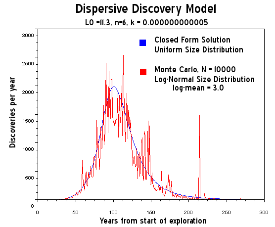
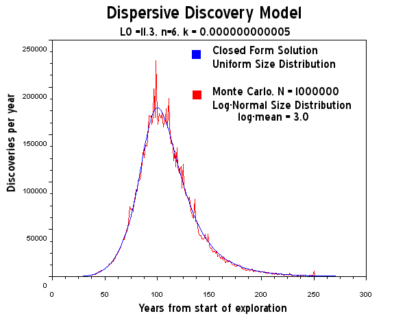
Figure 4: A discrete Monte Carlo simulation of dispersive oil discovery which shows both the statistical fluctuations and the sparseness of the finds down the tail of the curve. With more data sample the fluctuations diminish in size.

So contrary to recent activity of huge new discoveries as reported by the NY Times, the days of sustained discoveries remain behind us and we are seeing the occasional pop of the popcorn.

---

Ugo Bardi at TOD had posted a suggestion that we come up with a "mind-sized model" to described the Hubbert Peak. This makes a lot of sense as we still have the problem of trying to convince politicians and ordinary citizens of what constitutes the issue of peak oil and more generally peak oil.

Why we try to do this has some psychological basis. This last week, I worked on some ideas pertaining to the technique of Design of Experiments, and a colleague had turned me on to an in-house course on the topic. There, in the course notes introduction, the instructor had laid out the rules essentially describing the three stages of learning. The bullet points pointed out that understanding did not come about instantaneously, and instead progressed through various psychological stages. I figured that he did this as a precaution to not wanting to frighten his students at the level of effort required in learning the subject material. This explanation basically amounted to a cone of experience conceptual model, with a progression through the stages of enactive, iconic, and symbolic learning. Enactive amounts to a type of hands-on learning through first-hand experience; iconic boils it down to a psychological connection to the material via shared experience; and symbolic brings it to the level of analogies and potentially mathematics for the sophisticated learner.

The fundamental problem with understanding peak oil is that the enactive first-person learning and ultimately iconic shared experience only occurs on the most abstract level. We just cannot comprehend the global scope of the problem and can only reduce it to our day-to-day interactions and what we see at a local level. Therefore, only when we experience, or hear about something like gas station queues and price hikes do we make a connection to the overriding process at work. But these observations serve merely as side-effects and do not ultimately explain the bigger picture of oil depletion. In Bardi's view, it does not represent a good mind's eye view of peak oil.

Bardi tried to do this by comparing oil depletion to a Lotka-Volterra (L-V) model of predator-prey interactions. This works on all three levels, culminating in an abstraction that demonstrates the Hubbert Curve in mathematical curves. That would work perfectly ... if it actually modeled the reality of the situation. Unfortunately Bardi's L-V doesn't cut it and it will actually misrepresent our continued understanding of the situation. In other words, we cannot use Bardi's analysis as a tool for practicing depletion management. Our learning basically ends up in an evolutionary dead-end, and even though it effectively works on an emotional and psychological level to fill in our cone of experience, it misses the mark completely on mathematical correctness.

Other people try to make the symbolic connection by comparing the oil discovery process as searching through a pile of peanuts or cashews for edible pieces. This works on a qualitative level, but until we have some quantitative aspects, it ends up short on the symbolic mathematical level. I myself have used the analogy of finding needles in the haystack, which brings in the formal concepts of dispersion. The idea of popcorn popping fills in more of the enactive and iconic levels of our experience (who hasn't waited in agonizing expectation of the furtive last few pops?) and the experiments themselves demonstrate the symbolic math involved -- the process of accelerating discovery as our reserve bag of popcorn inflates, followed by a peak in maximum discoveries, followed by a slow decline as the most stubborn kernels pop. The production cycle culminates as we consume the popped popcorn at a later date.

To compare this understanding against Bardi's Lotka-Volterra or of the Verhulst formulations shows the limitations of the the predator prey model, as it simply does not take into account the stochastic environment of exploration. For example, what if we had applied an L-V formulation to the popcorn experiment, what would we get? Since it is deterministic, it would come out like a spike with the cumulative showing as a step function. All the L-V can do is work on the mean value, so that it misses the real dynamics of random effects. With L-V, all the popcorn would pop at the same time. This is as ridiculously simplistic an assumption as the spherical cow.

Moreover, the L-V model also assumes that some collective feedback plays a large role, as if the amount we have found or the amount remaining (as to in the Verhulst equation) determines the essentials of how depletion comes about. Yet, as the single kernel popcorn experiment bears out, the feedback term does not really exist. All we really have to understand is that certain stubborn pockets will remain and we need to keep accelerating our search if we want to maintain the Hubbertian Logistic-like shape. In other words, the natural shape does not decline as some intrinsic collective property. On an iconic level, the popcorn kernels that have popped don't tell their buddy kernels to stop popping once the bag is nearing completion. Yet, the predator-prey model tells us that is the reality and Bardi wants us to believe that interaction happens. That essentially what I want to get across: a real understanding of the situation.

So in effect, with the correct mathematical model, I could easily work out the popcorn dynamics from first principles and use that as a predictive tool for some future need (maybe I could go work for Orville Redenbacher). Or on a symbolic level, I would tell a politician that I could accurately gauge how long popcorn would take to pop and use that information to convince him that we could gauge future oil depletion dynamics. Unless he had never seen a popcorn popper in action (GHWB perhaps?) he would say, yeah that would make sense -- and then I could relate that to how it makes sense in how oil depletion dynamics plays out.

This is the kind of mind-sized model that we have just worked out.

---

Notes
[1] Apparently high school and college science teachers like to use popcorn popping experiments as a way to introduce the procedures of statistical data collection and the scientific method.

[2] A fixed exit criteria is like the finish line in a race (see below). A random exit criteria is where the finish line varies.