[[ Check out my Wordpress blog Context/Earth for environmental and energy topics tied together in a semantic web framework ]]

Tuesday, January 31, 2006

Bush hitting the everclear

If Bush gives ethanol the big push as predicted in tonight's SOTU address, that will provide the final nail in the coffin for ethanol's future. Has Bush gotten anything right yet?

Monday, January 30, 2006

Self-limiting parabolic growth

In the last post, I hinted that the parabolic growth law that oil reserve growth estimates seem to follow will likely hit some hard limit. After all, no one really believes in an infinite supply of oil .. do they?

I use the physical analogy of diffusion to come up with a model for reserve growth in this regime. In chemistry and materials science, engineers use the principle of diffusion all the time to estimate rates. A simple formulation, known as Fick's first law, supposes that the rate of material flow remains proportional to the concentration gradient across a range of spatial distances. This works ideally for conditions of fixed concentration with respect to time at the boundary conditions. Fick's second law makes the assumption that the concentrations can change over time, and a more complicated partial differential equation results.

Under the first law, the rate of transport (and therefore growth) tracks proportionally the concentration difference and inversely the distance between the opposing concentration layers. If the "growth" amounts to transferring material from one side of the layer to the other, the diffusivity D assists the flow from the high concentration area (C(0)) to the low concentration layer (C(x)), while the continued growth on the other side starts to retard it.
dG(t)/dt = D (C(0)-C(x))/G(t)


This flow becomes self-limiting only in the sense that it starts to progressively slow down. However, given enough time, diffusion happens and it will continue to grow indefinitely. In a material analogy, the oxides that form on silicon occur immediately and then start to slow down as the oxide gains thickness forming an increasingly impenetrable membrane. This gives the parabolic growth law -- perhaps better entitled the square root growth law -- which states that G(t) ~ sqrt(t).

The connection to oil reserve estimates mostly comes from making an analogy: that the geologists can only predict what they can measure, and they can measure the oil at the low concentration layer, having to wait decades for the high concentration layer to "diffuse" across the barrier. Admittedly, the "diffusion" I talk about may not symbolize real diffusion but rather a fixed difficulty in extracting material as we drill deeper, etc. We then will continually achieve diminishing returns, with an added real possibility of hitting hard limits.

Not wanting to work out the second law, but sensing that the concentration changes with oil depletion, I worked out a modification to Fick's first law whereby I changed the C(x) term to track the growth term G(t). This basically says that over time, the concentration differences start to level out.
dG(t)/dt = D (C(0)-a*G(t))/G(t)
Unfortunately, one can't find an analytical solution to this equation (except for the asymptotic behavior, which drops out straightforwardly). But, alas, we do have computers to do the grunt work of numerical integration. The following curve results for an a/C(0) ratio of 0.09 (the asymptote rather nicely goes to 1/0.09=11.1).

I plotted the 90-year reserve growth from Attanasi & Root (their "common monotone" data fit) on top of the curve so you can see one possible future extrapolation. Clearly, the enigma of miraculous parabolic growth starts to evaporate under this regime and extraction will continually eat away at the meager growth we will get in years to come.

And as I said in the previous post, I await eagerly the latest 105-year data updates from the USGS. This should conclusively show that the reserve growth curves level out as this model would predict.

Sunday, January 29, 2006

Backdating and reserve growth

In the USA, the government prohibits speculative estimates of the remaining oil in a field.
Operators in the United States are required by law to report only those reserves that are known with high certainty to be available for production, thus excluding resources that are at all speculative. It follows that one component of reserve growth is the difference between early estimates of recoverable resources, which in the presence of limited data are required to be conservative, and later estimates based on better knowledge of the field.
This means that oilers can't use the reserve estimate outlined in the previous post. That technique, which empirically demonstrates a growth of 10x or more from the initial estimate after 90 years, apparently ranks as a speculative estimate (blue curve below, assuming an initial growth estimator of 0.1). So, instead of coming up with an estimate based on established heuristics, the field operators always undershoot the actual amount, to safely remain below the "speculative" point.

That means that all the original discovery curves need continual updating, commonly referred to as backdating in the oil industry. I double-checked how well the oil-shock model (red curve above) tracked the average A&R reserve growth algorithm. The fit looks decent, with the cumulative production hanging below the parabolic growth at all points. If in fact my curve showed more than an order-of-magnitude tracking difference, I would worry that I seriously erred in my own parameter estimates and/or that the discoveries got backdated incorrectly. As formulated, the long lag in extraction comes about from the serial application of the fallow, construction, maturation, and extraction phases. These combine to a 1/e time constant of about 30 years, leading to the s-shaped curve shown.

The big problem with the A&R parabolic growth law remains unanswered. Although it does not show compound growth, neither does it show any signs of abatement -- as it should continue to grow for years according to the formula. As you can see, the oil shock model does hit a normalized limit at about the 90 year mark. I have only seen results for the A&R model up to the year 1991, with initial data from 1900. Which means it could show signs of abatement should anyone get the nerve to present more recent data from the last 15 years1. How about it USGS?

The Kuwaitis learned from the best in applying their own reserve growth estimates. I salute you, good ol' USA, for educating our foreign pupils. What a mess we have created.


1 This transcendental function follows a parabolic growth law initially, but then goes on to from an asymptotic limit, effectively stopping further growth.
df(t)/dt = K/f(t) - C*f(t)
I haven't checked the literature, but the parabolic growth law for oxidation should follow this behavior for very thin substrates where the source of materials limits out physically.

Friday, January 27, 2006

Grove-like growth

I looked at the dynamics of fossil fuel "reserve growth" some more and I do not think it demonstrates compound growth by any stretch of the imagination. If it did in fact show such behavior, the growth would fly off the chart in a Ponzi scheme fashion.

Compound growth in the traditional sense has a fixed proportional rate. This would give an accelerating slope. However, reserve growth has an apparently monotonically decreasing proportional rate over time which leads to a decelerating slope. Think of it this way -- if the growth rate follows 1/x, then any increase in x gets counterbalanced by a smaller proportional amount or ~(1+1/x)x. I plotted a 0.5/x curve (in green) on top of the moving-average fit below.

Having been away in Silicon Valley on business the past few days, I haven't had a chance to follow-up more quickly, but oddly enough, I sense an analogy to silicon in the way that reserve growth actually works. Andrew Grove, Ph.D. in chemical engineering, UC Berkeley, 1963, and a founder, current chairman and former CEO of Intel Corporation -- the world's largest maker of the silicon microchips that store and process information on computers. As a young Ph.D., Grove and his Fairchild Semiconductor colleagues helped create the modern silicon microchip by solving the problem of how to make silicon stable. The discovery helped revolutionize computer chip-making and gave Silicon Valley its name. Take for example, the work of Andy Grove, one of the co-founders of Intel, who did his PhD thesis in diffusion-limited oxide growth, a physical process critical to building integrated circuits. In a nutshell, silicon dioxide needs a source of silicon to form, but as the SiO2 layer gets thicker, it becomes harder and takes longer for the Si atoms to diffuse to the surface and react with oxygen. This leads to a law of the following form, where F(t) is thickness as a function of time:
dF/dt = k/F(t)
F = sqrt (2kt)
Note that the fractional rate reduces to:
dF/dt / F = 0.5/t
Note that this follows the "reserve growth" curve fit fairly well, where the fractional growth rate slows down inversely proportional to time. Microelectronics engineers refer to this as the parabolic growth law (a parabola sitting on its side, see the overlay on the green curve below).


Now if we suddenly became stupid semiconductor neophytes living in the 1950's and thought that the oxide growth could only be "guessed" at, then we would never have advanced through the microelectronics revolution and process unpredictability would have killed us. We would still be working with crystal radio sets. None of the multi-million gate circuits would have ever gotten made!

But the fact that material scientists and engineers like Andy Grove quickly characterized the phenomena within a few years time (mid 1960's) and got their process down to a gnat's eyelash speaks volumes about the difference between real engineers and the geologists who believe in magical, enigmatic reserve growth. (I don't know a fab engineer in a bunny suit who believes in "enigmatic" oxide growth)

I have a suggestion for the geologists and petroleum engineers. Figure out what the heck your measurements and estimates mean, and then perfect the formula to eliminate the magical guess work. The more I look at it, the more I seriously think that no one has figured out how to do estimates of oil reservoir volume correctly. Might they all measure the volume as an approximation to how much they have extracted, with the increase over time caused by diminishing returns? Much like a thick SiO2 layer prevents fast oxidation, that drilling "deeper" into a field slows further depletion and you need to work harder and wait on average longer times to get at it? It almost sounds as if no one wants to admit that a parabolic growth law has any kind of importance.

If done correctly, reserve growth would transform from enigmatic magic to a measure of extractability over time.

Monday, January 23, 2006

Reserve Growth Overrated?

At the urging of a petroleum engineer at the PeakOil.com board, I took a look at the Attanasi & Root approach to predicting reserve growth. I grabbed the oil field data from the journal below and OCR'd into something I could analyze (raw data here).
"Attanasi, E.D., and Root, D.H., 1994, The enigma of oil and gas field growth: American Association of Petroleum Geologists Bulletin, v. 78, no. 3, p. 321-332."

If I plot the raw data as a scatter plot which shows only fractional increases per year since the year of discovery it looks like the chart below. Note that this plot does not visualize the "multiplier" approach which A&R choose to do; IMO they do this rather unwisely, because it accentuates bad early estimates. The "fractional" approach provides an accepted statistical way to look at this kind of data which avoids amplifying regions with poor statistics.

I also put in a 20-point moving average filter to guide the eye (not weighted by size of field). Notice that in the sweet spot right in the middle of the chart, where we get the best statistics, the "reserve growth" fluctuates around 1% per year. You can see some growth for fields for fields older than ~80 years, but those have have worse sampling statistics than the rest. The latest data also exhibits poor sampling statistics.

Basically this approach demonstrates how you extrapolate assumed stationary data correctly.

Now, I ask the question how 1% reserve growth of mature fields will effectively compensate the 5% to 20% depletion rate per year routinely estimated for many fields?

Sunday, January 22, 2006

The Great Curve

This narrative describes the virtual flow of oil through the system from discovery to production, providing a problem domain description to how an oil peak occurs. You can find the accompanying stochastic differential equations here.

Precondition: Oil sits in the ground, undiscovered.
Invariant: The amount of oil in each of its states cumulatively sums to a constant.

The states of the oil in the ground consist of fallow, construction, maturation, and extraction.
  1. Someone makes a discovery and provides an estimate of the quantity extractable.
  2. The oil sits in the fallow state until an oiler makes a decision or negotiates what to do with it. Claims must be made, etc. This time constant we call t1, and we assume this constitutes an average time with standard deviation equal to the average. This becomes a maximum entropy estimate, made with the minimal knowledge available.
  3. A stochastic fraction of the discovery flows out of this fallow state with rate 1/t1. Once out of this state, it becomes ready for the next stage (and state).
  4. The oil next sits in the build state as the necessary rigs and platforms get constructed. This time constant we call t2, and has once again an average time with standard deviation equal to the average.
  5. A stochastic fraction of the fallow oil flows out of the build state with rate 1/t2. Once out of this state, it becomes ready for the next stage.
  6. The oil sits in the maturation state once the rigs get completed. We cannot achieve the maximum flow instantaneously as the necessary transport, pipelines, and other logistics are likely not 100% ready. This time constant we call t3.
  7. A stochastic fraction of the built rig's virtual oil flows out of the maturation state with rate 1/t3. Once out of this virtual state, it becomes ready for the next stage of sustained extraction.
  8. The oil sits in the ready-to-extract state once the oil well becomes mature.
  9. The oil starts getting pumped with stochastic extraction rate 1/t4. The amount extracted per unit time scales proportionally to the amount in the previous maturation state.
Post-condition: All oil eventually gets extracted at time=infinity. But because of the proportionality extraction rate assumed, this decline only asymptotically approaches zero at long time periods. Also, the cumulative amount extracted at time=infinity equals the total discovered. However, since we never achieve infinite time, cumulative extraction never matches cumulative discoveries.

We can consider each one of these states as a reservoir with a capacitive time lag associated with the time constant set for each stage. In stochastic terminology the flow approximates a Markovian Process.

The extraction from the final stage gives the average production level. Since Markov processes have well-behaved linear properties and remain conditionally independent of past states, we can apply an entire set of discoveries as forcing functions to this process flow and the result will reduce to a convolution of the individually forced solutions.

The final production profile over time approximates the classic Hubbert curve. This narrative explains in very basic terms how and why the peak gets shifted well away from the discovery peak. However we observe no symmetry in the derived curve, as the nature of time causality rules long negative tails out.


Regarding the US crude oil production curves, Staniford was able to make a very good fit over a few orders of magnitude using a gaussian. As for temporal properties of this curve over time, Staniford noted it has the property that:
   dP/dt = K * (t0-t) * P(t)

where t0=PeakTime. This relationship reads that the production increase slows down over time linearly, but also scaled by the amount in production at that time -- kind of an linearly decreasing positive feedback turned into a linearly increasing negative feedback. At t=t0, the production increase turns into a production decrease. Unfortunately, I can't provide a problem-domain narrative for the gaussian formulation. Like the logistic curve formulation, I get brain-freeze trying to shape it into intuitive terms.

Saturday, January 21, 2006

Markovian Process

We live in a stochastic world. The best prediction you can make with only minimal prior knowledge takes into account only the currently occupied state. That basically captures the essence of a first-order Markov process or property, which can describe the salient effects of many different phenomenon, everything from random walk to oil depletion. The process involves lots of little stepped events that collectively accumulate in a fuzzified fashion. It inexorably leads you in a direction, but the direction remains governed by largely randomly distributed events.

So leave it up to the old-school punk rocker Greg Graffin, PhD from BadReligion to capture it in song.
Markovian Process (Graffin)

You will all say that I am surely crazy
Only an unrepentant pessimist whose thoughts should be detained
But facts are sterile, not vulgar nor sublime
And they're not religion, they're for everyone
And signify the times
Today is a window, tomorrow the landscape
All you need to do is take a look outside
To know what we're bound to face
The level of disparity
The common man
The manner of destruction of the native land
The poverty of reprisal from all involved
And the scathing trajectory from the past
Markovian process lead us not in vain
Prove to our descendants what we did to them
Then make us go away

Friday, January 20, 2006

Cycle Killer

I live in an urban area, so you would think I would have an easier time getting around via pedestrian or bike power. Well, yes and no. I certainly have a number of roads to use and choose from; however, I run into enough man-made and natural obstacles to make navigation more difficult than it ordinarily should.

I plotted out the "fence" pattern I have to deal with in my several square mile vicinity in the annotated map below. Note that the star marks my home-base and the heavy white lines indicate fence-lines, with safe crossing points indicated by hashed gate markers.


It turns into a bit of a maze as nothing amounts to a straight-line shot unless I go directly south (forget about going west easily). Even though we have lots of streets, nothing becomes convenient if you can't navigate through the forbidden areas. The obstacles include freeways, creeks, rivers, railroad lines, golf courses, lakes, reservoirs, and stockyards. And then you get these hand-crafted zig-zaggy residential neighborhoods filled with cul-de-sacs, ostensibly designed to prevent undesirable from easily passing through. Including kids going to school, who in the end have no other choice but to take a bus.

I find it amazing how a supposedly mobile culture locks itself into such a rigid structure, with only the car disguising this fact. Able to compress both time and space by shortening perceived distances traveled, by spending our time driving we end up not noticing the barbed wire surrounding us. Alas, on a bike I see it all and want to strangle our short-sighted urban planners.

Thursday, January 19, 2006

This Must Be LaPlace

Through some straightforward math, I can create a closed-form expression for the stationary solution to the oil shock model. Note that this assumes constant values for all associated rates over time and a delta value for the discovery term. As a sanity check, the solution matches that of the gamma function in the special case of equivalent rates assumed during each phase.
F(t) = Discovery stimulus
R1(t) = Reserve emerging from fallow state, Rate = a
R2(t) = Reserve emerging from construction state, Rate = b
R3(t) = Reserve emerging from maturation state, Rate = c
R(t) = Reserve emerging from production state, Rate = d
P(t) = Production curve

The stochastic differential equations look like:
dR1/dt = F(t) - a*R1(t)
dR2/dt = R1(t) - b*R2(t)
dR3/dt = R2(t) - c*R3(t)
dR/dt = R3(t) - d*R(t)
P(t) = d*R(t)

This forms a set of linear differential equations. If we take the Laplace transform of this set and do the transitive substitution, we can get the production curve in s-space.
r1(s) = f(s)/(s+a)
r2(s) = a*r1(s)/(s+b)
r3(s) = b*r2(s)/(s+c)
r(s) = c*r3(s)/(s+d)

p(s) = f(s)*a*b*c*d/(s+a)/(s+b)/(s+c)/(s+d)
If we assume a single delta for discoveries, then f(s)=1. The inverse Laplace transform gives the following (unscaled) time-domain expression

For values of rates very near 2.0, the production curve looks like this:

Remember to make sure that no two rates identically equate or else the solution becomes degenerate as the multiple poles form singularities. I mention this because the formulation as shown should prove useful in an optimization setting. By scanning through the ranges of the set of (a,b,c,d) one can quickly zero in on a first-order fit for a known discovery date and corresponding production data.

Up to now, I have used a numerical integration scheme to solve these equations, but the straight derivation provides a bit of insight into how the phased time constants arithmetically combine the exponentials into forming the asymmetric production profile. However, the simplistic assumption of a delta discovery and constant rates prevent me from recommending the close-form solution for complex, highly-featured real-world production curves.

Wednesday, January 18, 2006

More Songs About Oil and Gas

--Update: A Pilgrim's Progress--
I have several objectives for my approach to modeling fossil fuel depletion, any one of which I don't mind achieving.
  1. Introducing something fundamentally new to the discussion.
  2. Going beyond the heuristics and empirical relationships that I see plastered everywhere, to an approach mathematically-inclined people can understand (the rub).
  3. Resurrecting some old but perhaps forgotten techniques buried in the literature (so far nothing has shown up, or has it?).
  4. Showing analogies to other physical processes, like an RC circuit in electronics or a 1st order damped system in mechanical dynamics.
  5. Using the formulation to historically analyze or make predictions based on current data.
  6. Demonstrate an alternative to and weaknesses of the conventional approaches such as the logistic curve and gaussian (questioning empiricism).
  7. Come up with an open-source modeling environment, where I can make all source code and data available to the public.
And above all, try to make the constituent parts fit together tighter than a litter of suckling piglets. Because therein lies the way to making progress in a purely meritocritous blogosphere.


So this blog entry once again contains categorized oil depletion modeling posts that I have written over the last half-year. By and large, I have proceeded from a micro world view to a macro view, while adding interesting details that help me gain insight into how other mathematically-inclined people understand our current Peak Oil predicament.
A Micro Peak Oil Model
Part 1 | Part 2 -- Stochastic analysis on the small scale

A Macro Peak Oil Model
Part 1 | Part 2 -- Stochastic analysis on the large scale

The Oil Shock Model
Intro | Continuous -- How disturbances affect depletion
RC Circuit (CAD simulation) -- Analogies to other processes
Code -- Generalized oil shock model program source code

And I have several posts which criticize the traditional Logistic curve but use the insight from the macro models as justification.
Issues with the Traditional Hubbert Model
Logistic vs Macro | Logistically Impossible | Logistic Curve Derivation | The Gamma Distribution | Peak Symmetry | Hubbert Linearization | Shock Model Linearization

Interspersed among the posts on mathematical formulation, I have tried my hand at fitting the shock model to historical stimulus and response data.
Fits to shock model using discovery data
Global using ASPO data (follow-up)
USA lower-48 (early Historical Fit)
UK North Sea (followup)
Former Soviet Union
Canada -- Weyburn
New Zealand Natural Gas, cliff
Norway
What ifs?
Can we delay peak by upping the extraction rate?
Calculating TOP (The Overshoot Point)
Monte Carlo Discoveries
Supporting information
Ramp-up data


Finally, some posts on the battles I have had with knowledgeable oil depletion deniers.
Reserve Growth | Creaming Curves | Framing | Desperation

Tuesday, January 17, 2006

Short timing

This helium-filled contraption may have a shorter life-span than the Hindenburg.

As natural gas supplies dwindle, and the accompanying helium reserves start to disappear, the military will likely have a hard time keeping the blimps aloft.


Whenever I see a proposal for a new vehicle with a bit of a retro makeover, I first cross-check against the art-work of Bruce McCall.

"By Zeppelin to Muncie"

Monday, January 16, 2006

Reserve Growth

A commenter at PeakOil.com referenced a paper on the "enigma" of reserve growth. I assume they call this an enigmatic phenomena in that no one really understands reserve growth and why it occurs. I have a few ideas, but first note a couple of things from the article. The authors work as consultants and hail from Canada. Does this color their outlook? Let's look at the charts. The first one shows a growth that appears fairly significant, perhaps an order-of-magnitude effect on reserve growth for oil and gas. However the second and third chart shows much more moderate growth.


But the first chart has a time scale that dates back 100 years. I don't have any idea of how they came up with this chart, but you have to ask: how effectively did the wildcatters estimate things 100 years ago? Is this the enigma -- that reserve growth doesn't appear as strong today as 100 years ago?

They also show another chart that has a big order-of-magnitude increase for heavy oil. What does heavy oil constitute in the USA and Canada? Can you say oil shale and tar sands?

A very muddled paper IMO. The authors haven't stated their results clearly, instead relying on innuendo and inferences. Fortunately they do show their data so that we can muddle our way through it as well.

A couple of apparently experienced oil people have contributed to the PeakOil.com thread mentioned above, ReserveGrowthRulz (a petroleum engineer) and RockDoc (a PhD geologist). I find it frustrating because they keep things close to the vest, alternately promising data and rationalizing things away with a sunny optimism. Take a look at this quote, which I highlighted:
ReserveGrowthRulz wrote:
Oh...I never said that ALL civilizations made the transition down through the ages from one energy form to another, just that us, as the human race, has done better in general, and succeeded in general, as we progressed through time and technologies.
In comparison to what? The orangutan race? The Martian race?

Face it, many of the petroleum engineers and geologists display hypocritical tendencies and thus can easily slide into a catch-22 situation. On the one hand, they can make these reserve predictions that err on the conservative side so that they can "grow" over time to make up for job insecurity. Fair enough, nobody ever got fired for underestimating a certain cash cow. But then they turn around and blame Colin Campbell and other oil depletion analysts for using the original and non-reserve growth numbers as proposed and continue to accuse them of "doomstering" because they keep missing the peak date. Of course you can perhaps fairly accuse Campbell of naivete in his estimates, but some deep-seated intellectual dishonesty prevents most everyone else in the oil industry from alerting us just why Campbell has made his own mistake of conservatism -- exactly the thing that the petroleum engineers practice and condone within their own profession.

So, 'fess up to where these "bad" numbers come from and we can take you geologists and petroleum engineers seriously. Right now I believe Campbell more than your brethren because at least he does not fly the flag of hypocricy.

I submit a suggestion on your road to redemption. Get rid of the euphemisms that call attention to the sunny optimism, and practice some honesty. As a first step I suggest that you don't call it "reserve growth", but instead refer to the issue as "bad estimate corrections". If you don't like that idea, I will give you a shovel and you can keep on digging a deeper hole.

Sunday, January 15, 2006

Linearization

The technique of Hubbert linearization for estimating oil URR works perfectly for only one class of models: those which obey the logistic curve. Although a linearization technique may apply for other models, the fact that no one uses other models likely means that one does not exist -- as of yet.

The fact that a logistic curve forms a straight line with negative slope if plotted as Rate/Q vs Q (where Q = cumulative), means that it gets a lot of head-nodding agreement when data seems to fit the linearization. Of course the oil shock model will not linearize the same way as a logistic curve will (as the curves themselves have distinct difference regarding symmetry, etc). In any case, I find it instructive to plot a typical delta-input (single discovery, all rates equal) oil shock depletion model with the same data transformation as the logistic curve.

If plotted on a semi-log chart, you can see the salient feature of the depletion model in a linearization context. At some point, further incremental additions of production will not affect the cumulative amount. This forms the oil extraction analog of "the law of diminishing returns".


Michael Lynch talks about (I think) linearization in his paper "The New Pessimism about Petroleum Resources: Debunking the Hubbert Model (and Hubbert Modelers)".

Concerning the above chart (Figure 4 in his paper), Lynch says:
Finally, Campbell and Laherrere use production data to estimate field size, "improving" on the IHS Energy data. By graphing production against cumulative production, as in Figure 3, they claim that a clear asymptote can be seen, allowing for a more accurate estimate of ultimate recovery from the field. The first problem with this is that there is no explanation for how often the method is employed.

[...]

Examining this data does confirm that some fields display a clear-cut asymptote. However, out of 21 fields whose peak production was above 2 mt/yr (or 40 tb/d), only 7 show such behavior. The rest do not show a clear asymptote (as in Figure 4), or worse, show a false one, as Figure 5 indicates. Clearly, this method is not reliable for estimating field size.
I see the problem in that Lynch does not plot the curve in the classical Hubbert sense, i.e. he forgets to divide production by cumulative along the vertical-axis. So basically, once again, either (1) Lynch gets something horribly wrong, or (2) the traditional analysts have become lazy in not rigorously using the Hubbert linearization, forcing Lynch to call them on it. Somebody may yet sort this out.

So what happens if we plot Lynch's Figure 4, the UK North Sea Cormorant field, the correct way? It looks like this:

Conclusion: It may not obey a true Hubbert linearization but it sure looks similar to the oil shock model along much of its range. If we plot the same delta-function driven shock model in the same way as Lynch does, it looks like:


Now, take a look at some of the other curves in Lynch's paper:

Kind of spooky? Look at the superposition of the curves.


Update: For yucks, here is another shock model with the first two time constants (Fallow period and Construction period) removed. This tends to make the curve more asymmetric and brings the peak in closer. (I gave all these curves the intuitive eyeball fit. And I normalized the curves by eye as well, since I had no discovery data.) Overall, I think this kind of "integration" linearization has some validity but it does transform data by compression, which tends to make the fit look better than if we kept the time domain in there and fit the original data as an "uncompressed" set of points. In essence, using the cumulative as an axis does a good job of filtering via integration, as discussed in a PeakOil.com thread. And the same holds true for Hubbert Linearization.

Friday, January 13, 2006

RockDoc gets piled high and deeper

rockdoc123 wrote:
Quote (me):
And will this get out to the textbooks? Or will it get buried like the rest of the stuff, until we all say "Wha' Happ'n?
having a black helicopter tin foil kind of day are we? There is reams of views on what is left to be found in the literature, has been since the seventies. Check American Association of Petroleum Geologists Bulletin, Bulletin of Canadian Petroleum Geology, Petroleum Geology, USGS Energy group assessment, etc.
I responded:
I will lay this out very carefully because my concerns involve a combination of the practice of "framing" along with negation of arguments that the industry condones via paid consultants. First consider how Mike Lynch has become one of the most visible debunkers of peak oil theory out there. And what does he use as ammunition? Lynch uses the mathematical formulation of Hubbert curves to allow peak oil advocates to effectively shoot themselves in the foot.

How does he do this? Well, he starts with the Logistic and Gaussian curves that the traditional analysts use and starts poking holes in how they get formulated. His favorite argumentative weapons include "physically impossible symmetry" and "causality violations". The argument about symmetry stands out because all one has to do is look at real-world depletion curves and see that most do not display any symmetry. Lynch points out that the curves should not be symmetric based on his own studies. Yet, depletion modelers continue to use them. Score: Lynch 1, Modelers 0

Lynch's causality argument says that the Logistic and Gaussian curves have tails at time 'minus infinity', which remains a physically impossible condition considering that humans only discovered oil in the mid 1800's. Peak oil analysts have nothing to counter this other than some magical truncation that occurs in the curves, without any supporting explanation. Score: Lynch 2, Modelers 0

Now, I would consider these minor blemishes on the overall peak oil theory, but Lynch builds a strong rhetorical argument building from this foundation of negating theories. This paper provides a good example of how he pulls together the arguments: "The New Pessimism about Petroleum Resources:Debunking the Hubbert Model (and Hubbert Modelers)". Lynch probably enjoys doing this and probably feels better than out-and-out lying about things (kind of the same reason that people don't cheat at crossword puzzles). Lynch probably just sits back and laughs in the way he uses the exact models as taught to petroleum engineers and geologists (as you just admitted, RockDoc), and then basically shreds and decimates the arguments. Listen again, the stuff you got taught in textbooks (Hubbert curves, etc) gets turned upside down and used by Lynch to "disprove" peak oil or at least cast suspicions into its relevancy.

Why does this work? You just have to look at the psychology of people and their fierce need to believe in the status quo. Any bit of debunking is enough to set the whole theory to collapse in these people's minds, especially the sharp ones (and former high-school debaters), who tend to revel in such nit-picking matters. A bit off-track but think back to how GW Bush's entire questionable National Guard record became vindicated when rabid right-wingers exposed a set of fraudulent memos. Even though the majority of the evidence pointed out that Bush avoided most of his service, the few flaws in evidence presented sunk the entire investigation. And we have a corrupt Bush administration as a result.

What can we do about this? (not Bush, I mean) Simple. Come up with better models than the Logistic curve or the Gaussian. These basically show empirical relationships that prove nothing and provide no foundation for understanding. Instead, teach something that works. Do you realize that an EE professor would be laughed out of a classroom if he showed a Gaussian curve as the output to a electrical circuit? Yet this figuratively happens when the Hubbert modelers keep on showing Logistic or Gaussian curves. I groan at the bad math, while Lynch calls them on the B.S. But the Campbell's and Laherrere's would never, ever give up their dearly loved Logistics formulations because of their selfish pride. Lynch counts on this as well; that they will keep on showing the Logistic curves and Lynch will keep on debunking. Lynch has basically framed the Hubbert modelers as inept mathematicians. Jeez, even CBS gave up their inquest when they could not counter fraudulent memos.

I say let's turn it around and call Campbell and Laherrere on their own models, and get some decent ones -- models that don't violate causality. Then we can effectively ignore Lynch, because he will have no legs to stand on. Or else, he will eventually resort to out-and-out lying and we can call him on that.

Rockdoc, What you call "tin-foil hat" theorizing on my part basically ignores and discounts the modus operandi of the entire right wing corporatist establishment. If we can just beat down the framing and negative arguments practiced by consultants like Lynch, we might have a chance to stop digging a deeper and deeper hole.

Or you can laugh and pass my whole approach as a phony strawman. But then you have to remind yourself of who we have as president. This framing stuff works and you may have drunk the kool-aid.

Thursday, January 12, 2006

Oil companies don't do depletion modeling, or they did at one time but now just don't care

Compared to the clueless petroleum engineer featured in yesterday's post, the geologist rockdoc takes a measured view of things. He remains optimistic and offered up some thoughts on my depletion modeling approach here. However, I still get frustrated because of the casually dismissive attitude that big oil has apparently indoctrinated into anyone that gets within a 10-ft pole distance of their clutches. I annotated his musings with my own rhetorical questions in the following snippet:
rockdoc123 wrote:
WebHubbleTelescope...what you just created as I remember was being used some twenty years ago in the research labs (back when oil companies like Gulf and Shell had large research facilities and had no problem hiring people with a maths jones to sit in an office and fiddle with data).
So why did not such a fundamental analysis get transferred to the textbooks? The lack of this kind of analysis is much like teaching first-year electrical engineering without introducing Kirchoff's Law. It's just freaking rate equations and conservation of matter. This to me is deeply troubling. I didn't take an earth sciences major, but I have taken classes in subjects such as limnology and the first thing you learn is that all freshwater lakes go through a life-cycle, birth through death. Are the petroleum engineering departments so vain and self-conscious not to even broach the subject of the life-cycle of oil? To avoid teaching that the whole thing is just a house of cards or a ponzi scheme, certain to eventually collapse, strikes me a bit irresponsible.
rockdoc123 wrote:
Today most oil companies are just not that interested in how much might be left overall (exception would be BP who still has a pretty big research component)...they spend their time modeling existing production and coming up with predictions on whats left to be discovered in various parts of the world where they are working.
And will this get out to the textbooks? Or will it get buried like the rest of the stuff, until we all say "Wha' Happ'n?"
rockdoc123 wrote:
This sort of analysis involves more subsurface information and requires less math analysis of past trends. If memory serves me correctly some of the old analyses were published in the AAPG Bulletin.
OK, so this got published. How about the results from 20 years ago?
rockdoc123 wrote:
It would be interesting to look at the same analysis for somewhere other than the US.
I have analyses for North Sea, World, lower-48, even for natural gas.World | Lower-48 | UK North Sea | Former Soviet Union | New Zealand NG | Norway

I use the same model for everything, vary the parameters a bit, and gain an understanding that I surely would not have if these rate equations were not available. We could be mining for marbles, it doesn't really matter, I see no fundamentals being taught or published anywhere. The more I look at it, this stuff with the Logistic curve and Gaussian fitting is basically rubbish. It's equivalent for me to trying to teach the response of analog electric circuits by looking at the output waveform. I would like to see the oil depletion modeling rise a step above shear empiricism.
rockdoc123 wrote:
Arguably the US has been a poster child for making discoveries and getting them on-stream with little in the way of interuption or government imposed obstacles.
Government-imposed obstacles seem like a second-order effect when put up against the greed of the human animal. Teach the first-order effects first. Just about everything in engineering is first -order effects. If you don't do the first-order stuff first, you should just give up. They don't call it first-order for nothing.

I also think it important to do this fundamental kind of analysis to prevent the Michael Lynch's of the world to continue to drive a tar sands truck through the occasional gaps in the logic of conventional oil depletion analysis. You basically have to get rid of all of the logistic or gaussian curve fitting arguments or you will fall into Lynch's favorite tautology traps -- notably that of impossible symmetry and causality violations.

Most of the people on the oil depletion sites seem to want to hang on to their belief in the logistic formulation, and so Lynch will continue to eat their lunch, in a figurative sense. Lynch has it wrong of course, but his arguments amount to a perfect framing that every right-wing political tactician would be damn proud of. A commenter at TOD mentioned the technique of "psychological and/or language patterning". Whether the oil companies actually fund Lynch, Yergin and others, I don't really know, but if they did it would make an effective 1-2 punch.
  1. Withhold information, both data and analysis
  2. Hire consultants and political cronies to run interference and obfuscate.
Hey, if it works in politics...

Wednesday, January 11, 2006

Don't let your babies grow up to be petroleum engineers

Over at peakoil.com, someone posing as a petroleum engineer made this rather optimistic claim:
ReserveGrowthRulz wrote:

Depletion alone is only a part of the overall dynamics which go into worldwide production rate, without accounting for new discoveries, their sizes and future rates, old fields changing their depletion profile through better technology and reserve growth, new areas opening up to exploration as, say, the Arctic seapack melts and makes more areas available, without including all of these it would seem to me depletion modeling exclusively is kinda like closing your eyes, grabbing an elephant by the tail and trying to describe his size off of what you've got in your hand?
Upon which, I responded:
Using the melting Arctic seapack as a rationalization for anything strikes me as a last gasp attempt at maintaining the status quo.

Cripes, if the seapack starts to melt at rates at which we need to replenish our oil supply we have a whole "boatload" of problems to start worrying about.

To which he countered (apparently showing no sense of irony):
Arctic ice melting opens up areas of exploration that haven't been available before, both practically and economically. The USGS numbers for undiscovered resources for Greenland are a perfect example, they say maybe there is a little, but maybe there is ALOT.

Spending ALOT of time on the internet there, huh? When did the oil companies start hiring these loosers? I guess they made up some new rulz for the flood of cronyist appointments and their offspring.

Tuesday, January 10, 2006

Creamed again

One of peak-oil denier Michael Lynch's favorite arguments to counter the oil depletion pessimists out there (Campbell and Laherrere, et al) has to do with questionable interpretation of the so-called "creaming curves" from mature fields. Since I did some real honest-to-goodness Monte Carlo simulations fairly recently, I think I have a handle on what Lynch has gone half-cocked over. Bottom-line: nothing to get excited about -- just Lynch practicing his highly refined art of attacking the model and not the reality of the situation.

Lynch essentially states that the creaming curves that get published have a tendency to creep up over time, implying that more oil exists than anyone currently realizes. I have thought about this for awhile, found his arguments somewhat intriguing myself, until the trickery finally popped into my head. Unfortunately, Lynch has mistaken the asymptotic properties of finite regions with the semi-infinite scope that some creaming curves occur under.

As an example, consider this Lynch curve:

Note that one curve gets plotted according to time progression. From the looks of it, it doesn't appear to have any asymptotic properties. On the other hand, when ordered by size (i.e. sorted), it shows a clear asymptote. Lynch likes to point out that people shouldn't look at the purple curve because the other one keeps climbing. What Lynch fails to point out, and many people have gotten taken by, constitutes a rather serious sin of omission on his part. He doesn't state his assumptions. If he did, then you would see the flaw in his argument rather quickly.
  1. Within a finite field area, the asymptote gets truncated artificially. The geologists or petroleum engineers declare the field "dry" when they stop finding strikes, go back and order the numbers, and figure out the creaming value. Ordering the values high to low and doing a cumulative sum gives the curve a filtered look that shows a horizontal asymptote. Graphically displaying the integration works out as a nice PowerPoint slide for management. The men in the suits agree, nodding their heads, and go on to the next field. And the engineers and scientists don't have to try to suck blood from a turnip.
  2. Within a quasi-infinite or continuously expanding field, the asymptote continues to creep upward. You can't make any assumptions on asymptotic behavior because the big discovery occasionally occurs, pushing the curves inexorably upward. In reality, only when you hit the limits of your quasi-infinite world can you make any serious interpretations on creaming.
The moral: Unless the field has hit the end of its lifetime, don't read too much into a creaming curve. If the discoveries do follow an ordering according to size, big to small, you might have an argument to stand on. (The unsorted curve should show show a noisy but quite straight linear upward trend if the sizes show independence with respect to time) However, in the quasi-infinite situations, the big discoveries will likely still occur where you haven't looked, thus invalidating any asymptotic trend that you may have counted on.

This exercise in Lynch de-debunking helped me see another interesting property of the creaming curve. When ordered according to size, a histogram of the individual slope values gives the probability density function. Which means you can easily check against a log-normal distribution. If I could find a creaming curve for the entire world, we should get a good distribution to work with.

Monday, January 09, 2006

Would You Believe?

In my previous post, I made an offhand reference to how the initial increase of crude oil discoveries might follow a certain well-understood pattern:
I then put a "gold rush" mentality on the frequency of discovery strikes; this essentially started with 8 strikes per year and rising to 280 strikes per year at the peak.
You can either think of the discovery growth as a steady year-to-year increase or as an accelerating increase. The latter refers to a quadratic growth law commonly found in many situations where increasing numbers of resources get applied to a problem over time. Much like gold spawns a fevered rush of interest which seems to accelerate through a parabolic boom before finally busting, I offer that oil strikes might follow the same swarming pattern.

Consider a very recent example of quadratic growth which comes from the wonderful world of the Wiki. At least one team of academics has noticed that the rate of increase of Wikipedia words follows a quadratic growth law. I extracted the following relationship from the Wikipedia statistics table:

Note that when we take the square root of the growth, it tracks a straight line. Also remember that quadratic growth does not equate to exponential growth. Exponential growth occurs when the rate of increase of a quantity proportionally scales to the amount of quantity at that specific time. This amounts to a much different swarming activity.
Quadratic Growth : d2Q(t)/dt2 = k
Exponential Growth : dQ(t)/dt = aQ(t)


In the context of crude oil discovery, I curiously haven't seen much written about the number of discoveries over time. From my last post you can clearly see how noise obscures much of the trend (which the oil shock model effectively filters out -- more on that in a future post).

However, over the weekend, Staniford at the TOD blog brought up the topic of USA production curves dating back to the first discovery made in 1859. He created some quite amazing fits to the entire USA oil production profile using a gaussian function, which looks like an inverted parabola on a semi-log plot:

That particular parabola, a quadratic in fact, I have little interest in. But, I do get excited about encountering some new data to pound on.

I used the USA lower-48 discovery table as a reference point and then eyeballed a quadratic growth factor to generate an accelerating rate of oil discoveries.

The discovery peak hits about 1930 and then decreases after that point -- basically a boom and bust cycle in full view.


With the basic assumption that the size of strikes remains independent over time, I took a shot at applying the oil shock model to the artificially constructed quadratic discovery data. I used about the same extraction rate that I previously used for the lower-48 model increasing it slighty to 0.08. I modified the fallow, construction, and maturation constants a bit from 8 years to 12 years. I did not apply any oil shocks, because they would not show up on this kind of scale in any case. I just wanted to see if I could match that gaussian characteristic that Staniford observed.

I will let you pick the winner. Note the EIA data points from 1859 and 1860 that Staniford omitted because he considered them "outliers".

As an assumption I had to give the model an initial discrete stimulus to promote the discovery value above zero in 1859 (alternatively, I could have backed up the starting point a bit). This transient has little effect other than to keep the numbers on the graph. However, you can see that even the real data seems to plunge toward zero at the discovery -- something that the gaussian curve cannot handle. (Some people treat outliers as garbage, I prefer to treat them with a modicum of respect :-) Moreover, as I pointed out on the TOD comments, the extrapolation of the gaussian would show 100 of barrels of oil in production many years before somebody officially discovered the oil! In other words, the gaussian curve does not consider causality correctly.

Interestingly, the initial point that the EIA gives, 5000 barrels, has a lengthy historical narrative.
On a brilliant Saturday afternoon, August 27, at 69 feet down, the drill suddenly dropped six inches into a crevice. Uncle Billy fished it out, wiped it off carefully, and knocked off for the Sabbath. But Monday seemed a long way off, and on Sunday Smith was back at the well, peering down the pipe, wondering if he really saw something glistening on the surface below. He grabbed a leftover end of pipe, plugged it up like a dipper, and thrust it down on a stick. It came back up filled to the brim with oil. A wild shout brought several mill hands running. Young Sammy raced off to town to notify Colonel Drake.

The whole village was buzzing; even townsmen who still couldn't imagine what might come of the find were eager to see it. A man from the nearby town of Franklin, on the Allegheny River, who visited Drake's well the following day, joining the eager crowds streaming in on every road in wagons, on horseback, and on foot, reported, "It comes out a flowing dark grease with a heavy white froth."

By then, the few pine barrels Drake had provided were already full. Drake took Margaret Smith's washtub from the engine-house shanty (she complained later she never could get it clean after that), then commandeered old whiskey barrels and sperm oil containers. And still Uncle Billy kept pumping and the oil kept coming; so did the crowds.
The story also gives some older historical background. I did not know this, but arguably, we shouldn't even attach the discovery of oil in Titusville to any individual person. Many settlers had seen the residue in the oil over the years. So yes, in fact, it likely showed a fallow period, followed by Drake's construction period, and finally a maturation period.

Funny how things scale.

Saturday, January 07, 2006

Monte Carlo Discoveries

I learned moons ago in engineering school that you should not fear noise. Noise can actually tell you a lot about the underlying physical character of a system under study. I started thinking about this again because of the historically noisy oil discovery curves that 
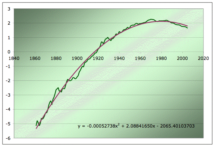
get published. This chart of global discoveries appears unfiltered:

This chart I used in the past has a 3-year moving average:

Some say that the discovery curves approximate a bell curve underneath the noise but I would differ with that assertion as the noise still exists even with a moving average applied. From the Schopper's article above:
"Pearson's r" test found no correlation between oil discoveries from one year to the next, i.e. discoveries appear to be random.
The fluctuations become very apparent because of the limited number of discoveries we have had in a finite amount of time. Laherrere estimates that worldwide we have had on the order of 10,000 crude oil discoveries. Pepper this over a range of 100 years and you get a relatively small sample size to deal with per year. This small number over a span of <100 years essentially gives rise to the relatively big yearly fluctuations. Making it even worse, we still have to consider the distribution of resorvoir sizes; anything that shows a large variance in sizes (i.e. a spread) will lead to larger fluctuations.

The reservoir size distribution seems to follow a log-normal function, which has the nice property of preventing negative sizes by transforming the independent variable by its logarithm (i.e. logs of the values follow a normal distribution). This pattern also seems to work for natural gas reservoirs:
Lognormal distributions -- a method based on the observation that, in large well-explored basins, field-size distributions approximate to a lognormal distribution. The method is most reliable with large datasets, i.e., in mature basins, and may be unreliable with small datasets.
As the variance tightens around the mean, the shape of the curve peaks away from zero. But importantly, a large variance allows the larger-than-average sizes (the "super-giants") to appear.


The physical basis for a peaked distribution (away from truly small sizes) likely has to to with coalescents and agglomeration of deposits. Much like cloud droplet and aerosol particulate distribution (which also show a definite peak in average size due to coalescence), oil deposits have a similarity in structure if not scale that we can likely trace to fundamental processes.

With that in mind and spurred on by comments in a recent TOD post:
The area under the complete discoveries curve must equal the area under the eventually completed global production curve, whatever it's math description - oil discovered must equal oil produced. The discovery process is controlled heavily by the math laws of probability with the bigger, easy-to-find pools of oil found first. Resource discoveries fall on bell curves too. Deffeyes makes the point that even with changing technology, this is the way discoveries play out. The global discoveries curve peaked in the mid 60s and, despite the immense tech revolution since then, the charted yearly discoveries have formed a pretty nice fit to a Gaussian bell curve, particularly if they are "smoothed" by grouping into 5 year bars in a bar graph.
I decided to take a shot at running a Monte Carlo analysis that shows the natural statistical fluctuations which occur in yearly discoveries. This data comes from several Monte Carlo trial runs of 10,000 samples with a log mean of 16 (corresponding to 9 million barrel discovery), and a log standard deviation (corresponding to 0.73 million barrel on the low side and 108 million on the high side). I then put a "gold rush" mentality on the frequency of discovery strikes; this essentially started with 8 strikes per year and rising to 280 strikes per year at the peak.

The first chart shows a typical sample generation, and the rest generate the discovery curves via the application of a steadily rising and then falling yearly accumulation factor; i.e. without the noise it would look like a triangular curve.


The main thing to note relates to the essential noise characteristic in the system. The fluctuation excursions fairly well match that of the real data (see the first diagram at the top of this post), with the occasional Ghawar super-giant showing up in the simulations, at about the rate expected for a log-normal distribution. But the truly significant observation relates to the disappearance of the noise on the downslope, in particular look at the noise after about 1980.

Remember what I said initially about noise telling us something? The fact that the noise starts to disappear should make us worry. That noise-free downslope tells us that we have pretty effectively mined the giants and super-giants out there and that oil exploration has resorted to back-up strategies and a second pass over already explored territory or to more difficult regions that have a tighter distribution of field sizes.

Contrary to the TOD commenter, I wouldn't quite say that the biggest fields get discovered first (Schoppers also sees no correlation), only that they have a higher probability cross-section which overcomes their naturally lower frequency of occurrence. The big ones may actually be found later because, over time, more resources get applied to exploration (increase in number of darts thrown at the dart board). And then eventually the resources get applied to more difficult exploration avenues as that dries up. That basically accounts for the noisy rise and noisy fall, until the noise disappears.

--

So we can largely account for the noise. The real smoothing process comes about when we apply extraction to these discoveries, essentially dragging the data through several transfer functions that extracts at rates proportional to what is left. This does not result in a logistic curve, but something more closely resembling the convolution of the discovery data with a gamma distribution. Which leads us full circle to the basis for my oil shock model.

Update: A thread over at PeakOil.com has the optimistic yet open-minded RockDoc commenting:
Remember that the Megagiant field size sits on the 99 percentile of world field size distribution….meaning that the chance of finding another is pretty slim.
As to the likelihood of finding more of them diminishing every day….that is only true if exploration efforts in areas where they are most likely to be found has been aggressive.
The RockDoc, an industry insider, promises to provide some data after I maniacally ask "I propose that rockdoc volunteer what he thinks is the global log-normal distribution of discovery sizes".
I think I can do that...I have a nifty program that will plot out field size on log normal probability paper. May take some time to dig up the field sizes though (I think I have it up to 2003 but may not have the 2004 data yet)....I'll first check to see what is in print already. There are some problems in doing this though...as an example Ghawar is often treated as being one big accumulation when in fact there are several distinct pools...hopefully that will be lost in the noise.
We'll see what he comes up with. He better get it out quick before every single internet transmission gets filtered by corporate legal departments courtesy of BushCo.


Thanks to Aldert Van Der Ziel, "Professor der Noise", who I had the privilege to study under in grad school.
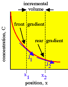
Friday, January 06, 2006

Teachy feely

Staniford has a new Hubbert Linearization post up at TOD. I still don't feel that approach merits any worth, but many people feel differently; from a commenter at the site:
It doesn't seem to be out of the realm for this to be taught in college/grad school to a fairly broad audience. Why has this been held back so long?
I can answer that. Because this particular approach resorts to a grab-bag of heuristics and empirical relationships and does not rise far above mere fortuity. Staniford says hisself that
" (I confess that I still don't fully understand why this model works as well as it seems to in practice)"
Placing myself in such a situation, I wouldn't feel comfortable teaching anything I don't deeply understand to a bunch of hungry graduate students. On the other hand, I would feel perfectly fine teaching the oil shock model, because of its reliance on some physical reality and the properties of stochastic processes.

Thursday, January 05, 2006

A Setup

I think Kevin Drum set up his readers with this post regarding a solution to global warming, caused by decomposing agricultural waste:
Take advantage of that. The leftover corn cobs and stalks from our fields can be gathered up, floated down the Mississippi, and dropped into the ocean, sequestering it. Below about a kilometer depth, beneath a layer called the thermocline, nothing gets mixed back into the air for a thousand years or more. It's not a forever solution, but it would buy us and our descendents time to find such answers. And it is inexpensive; cost matters.
The catch, as succintly revealed in the comments:

corn cobs float


Don't ever ask Kevin to dispose of the bodies. Ask a Republican instead. They would know enough to make sure to tie little lead weights to each of the cobs.

Wednesday, January 04, 2006

Norway offshore depletion

I gave a shot at modeling the Norway depletion curves starting from the Laherrere discovery data.

In the oil shock simulation, I used means of 5 years for the fallow, construction, and maturation periods, and a 10% depletion rate for years up to 1992. After 1992, like for the UK, I doubled the extraction rate over a 10+ year period. The fit is decent and it gives much more insight than the questionably derived logistic curve formulations.

Unshocked -- 10%


Shocked -- 10% to 20%


Note how close the profile of the shock perturbation approaches that of the UK North Sea model (chart to the right). In both cases, the increases in extraction rate occurred right around 1992, and essentially targeted the same 3 MBls/day sustainable production rate (competitive pressures perhaps?).

Like in the UK, the Norway model shows how the offshore areas can suffer rapid depletion. From the range of the parameters, the Brits developed and matured their rigs much more quickly than the Norwegians. The necessary increase in the extraction rates as the production curves started leveling off in the early 1990's became quite obvious; this basically forced the hands of each of the producers to pump harder. Without new discoveries, and continuous hammering on the extractive technologies, they will certainly see a steep decline before they put the expensively maintained rigs into mothballs as the North Sea oilers cut and and run and forever minimize their losses.

I got motivated to run this simulation from a thread on the PeakOil.com message board.

Update: Apparently, those in the oil industry call this falloff by the phrase pump and dump because of the high cost of extraction [link].

Fallout

If media reaction serves as an indicator of the outrage, I would presume that we will soon hear "more strip mining" as a safer alternative to coal mining. I predict the first talking points will come out of the Druggie Limbaugh show. His favorite whipping boys, the "eco-nazis" will become the target of blame for what happened in West Virginia.

Tuesday, January 03, 2006

Hovering for dollars

One day in and I have broken my resolution. This unsubstantiated quote by OILYROD follows up on a PeakOil.com message from last year in reference to the inventor of the SkyCar:

PostPosted: Wed Jan 04, 2006 7:41 am
Post subject: Re: Professor Paul Moller: Peak oil is a F#$%ing scam!

As a long time former employee of Dr Moller (AKA PT Barnum)I would like to set the record strainght.
1. He is not a professor at UC Davis, and hasn't been for over 15 years. He was never professer emeretus of anything.
2. He is in the business of taking peoples money, that's all. Shit, Burt Rutan got a plane into SPACE (twice) for about 20 mil. Where do you think PT has put the 50 to 100 mil he's duped folks out of?
3. The technology is impractical, and Mollers vehicles just don't work. The last test flight (30 sec and 15 feet up) was almost 3 years ago.
4. Moller has been making claims like today's for about 30 years. It's always "just around the corner". Google his name or "Discojet" and see what you come up with.
5. The only thing this guy is expert att is taking other peoples money.
Not surprising, considering his over-the-top resume.
When he was only 6 years old he began construction of his first house.
He likely obtained several technical degrees in utero as well.

Monday, January 02, 2006

"Oil executives don't drink whiskey"

I heard a spirited, yet civil, exchange on the Majority Report radio show on AAR tonight. The show featured a discussion between John Perkins (author of "Confessions of an Economic Hit-Man"), the hosts Janeane Garafalo and Sam Seder, and Janeane's father Carmine, who happens to have worked at Exxon in some capacity for the last 30 years. Carmine, somewhat of a staunch republican, apparently doesn't buy into the premise for Syriana, the depiction of oil executives thereof, the reasons for entering Iraq, etc. Janeane summed it up by saying something along the lines of "some people just don't want to know the truth, as it disrupts their belief system". For me, I still don't know whether Perkins plays up the snake-oil a bit too much, but nothing lately has negated any of his assertions. Perkins thinks the Iraq/euro connection created one rationalization for invading, yet Stirling Newberry thinks otherwise:
Fears about the US dollar - or about oil trading in Euros, are however, overblown. Instead, instability will help the dollar, as "flight to safety" will drive risk averse parked money here to the US. It doesn't matter what oil is traded in - the pound crumbled in the 1920's even though it was the unit of account for major commodities - but instead where the money is parked afterwards. Trading in euros will give Iran and other nations a hedge against another move on the dollar, but this is not significant. What is more significant is that there is a sharp willingness on the part of major dollar holders to move to Euro based stocks and bonds. The trigger point will be a European recovery. If europe can recover from its current economic slump, and raise rates, this will be a capital magnet. There are those that worry that this is destined to happen soon. However, the likelihood is that it will not happen until late in 2006 or early 2007, which means that the pressure on the greenback is still two years away.

The real tinderbox is not mechanisms, but control over the oil itself, and US attempts to keep nations that are oil holders vulnerable to US military pressure. ...
Of which Perkins acknowledged as well, in the context of China thirst for oil and their reliance on Iraq/Iran oil.

The Perkins segment starts in the second hour of the 3-hour program; the mp3 recording removes the commercials so you may have to scroll around for it: [MP3]

I end my vacation with a movie quote from the MR blog:
Three Kings (1999)

George Clooney's character: "I don't even know why we're [in the Middle East]."

character Ron Horn: "Don't start that with me."

Clooney: "Just tell me what we did here, Ron."

Ron: "What do you want to do- occupy Iraq- the new Vietnam all over? Is that your brilliant idea?"

and this from Pi:
Pi (1998)

Sol Robeson: "This is insanity, Max."
Maximillian Cohen: "Or maybe it's genius."

Sunday, January 01, 2006

Strip Mining of Parks

I had a chance to get some extra cross-country skiing in during the holiday break and came away with a sour taste from the decision making of the local parks and recreation board. A local park reserve called Elm Creek recently underwent "renovations" that amounted to lots of earth-moving activity. Most of the changes centered around the upgraded visitor center and I came away perplexed that I really didn't recognize the landscape that I had gotten used to over the last dozen or so years that I have visited the reserve. In particular I noticed a massive clearcutting of foliage on the main slope running down from the center to apparently make room for multiple grooved sledding runs. To me it looked more like a moonscape or a Fred Freakin Flintstone RV park.

I suppose someone had a rationalization for this (I have never seen the park so crowded), but if we can't avoid toying with the concept of a park reserve then we have little hope of avoiding a strip mining of our entire landscape in the quest for fossil fuels.

Like G. Bush and his ongoing fruitless quest with removing red cedar from his ranch, a significant fraction of the population has this strange innate desire to control their environment.
Bush showed reporters an injury to his forehead, a scrape from "combat with a Cedar" while brush-clearing at his ranch. "I eventually won. The Cedar gave me a little scratch," he said.
Won what? The battle? Or the war?

Update: The great Digby also ruminates on this man's obsession, which I think expresses insight into fundamental human nature.
So he clears brush like a madman everytime he gets the chance, hiding behind his Oakley's, blessedly unable to hear anything over the sound of chainsaws ---- maybe even the voices inside his head that remind him that he's still got three more years of this horrible responsibility he knows he cannot handle.