Application of the Dispersive Discovery Model

cross-posted from The Oil Drum (go there for a better formatted post)

Sometimes I get a bit freaked out by the ferocity and doggedness of the so-called global warming deniers. The latest outpost for these contrarians, climateaudit.org, shows lots of activity, with much gnashing over numbers and statistics, with the end result that they get a science blog of the year award (a 1^st place tie actually). Fortunately, the blog remains open to commenting from both sides of the GW argument, which if nothing else makes it a worthy candidate for some type of award. Even though I don't agree with the nitpicking approach of the auditors, they do provide peer review for strengthening one's arguments and theories. I can only hope that this post¬ on oil depletion modeling attracts the same ferocity from the peak oil deniers out there. Unfortunately, we don't have a complementary "oil depletion audit" site organized yet, so we have to rely on the devil's advocates on TOD to attempt to rip my Application of the Dispersive Discovery Model to shreds. Not required, but see my previous post Finding Needles in a Haystack to prime your pump.

Figure 1: Reserve size distribution pyramid

A Premise In Regards To The Pyramid

I start with one potentially contentious statement: roughly summarized as "big oil reserves are NOT necessarily found first". I find this rather important in terms of the recent work that Khebab and Stuart have posted. As Khebab notes "almost half of the world production is coming from less than 3% of the total number of oilfields". So the intriguing notion remains, when do these big oil finds occur, and can our rather limited understanding of the discovery dynamics provide the Black Swan moment¹ that the PO denialists hope for? For a moment, putting on the hat of a denier, one could argue that we have no knowledge as to whether we have found all the super-giants, and that a number of these potentially remain, silently lurking in the shadows and just waiting to get discovered. From the looks of it, the USGS has some statistical confidence that these exist and can make a substantial contribution to future reserves. Khebab has done interesting work in duplicating the USGS results with the potential for large outliers -- occurring primarily from the large variance in field sizes provided by the log-normal field size distribution empirically observed.

But this goes against some of the arguments I have seen on TOD which revolve around some intuitive notions and conventional wisdom of always finding big things first. Much like the impossibility of ignoring the elephant in the room, the logical person would infer that of course we would find big things first. This argument has perhaps tangential scientific principles behind it, mainly in mathematical strategies for dealing with what physicists call scattering cross-sections and the like. Scientifically based or not, I think people basically latch on to this idea without much thought.

But I have still have problems with the conventional contention, primarily in understanding what would cause us to uniformly find big oil fields first. On the one hand, and in historic terms, early oil prospectors had no way of seeing everything under the earth; after all, you can only discover what you can see (another bit of conventional wisdom). So this would imply as we probe deeper and cast a wider net, we still have a significant chance of discovering large oil deposits. After all, the mantle of the earth remains a rather large volume.

On the the same hand, the data does not convincingly back up the early discovery model. Khebab's comment section noted the work of Robelius. Mr. Robelius dedicated graduate thesis work to tabulating the portion of discoveries due to super-giants and it does in fact appear to skew to earlier years than the overall discovery data. However, nothing about the numbers of giant oil fields found appears skewed about the peak as shown in Figure 2 below:

Figure 2: Robelius data w/ASPO total superimposed

Figure 4: Shell Oil data

Figure 3: Discovery data of unknown origins

As is typical of discovery data, I do spot some inconsistencies in the chart as well. I superimposed a chart provide by Gail of total discoveries due to ASPO on top of the Robelius data and it appears we have an inversion or two (giants > total in the 1920's and 1930's). Another graph from unknown origins (Figure 3) has the same 62% number that Robelius quotes for big oil contribution. Note that the number of giants before 1930 probably all gets lumped at 1930. It still looks inconclusive whether a substantial number of giants occurred earlier or whether we can attach any statistical significance to the distribution.

The controversial "BOE" discovery data provided by Shell offers up other supporting evidence for a more uniform distribution of big finds. As one can see in Figure 4 due to some clearly marked big discoveries in the spikes at 1970 and 1990, the overall discovery ordering looks a bit more stationary. Unfortunately, I have a feeling that the big finds marked come about from unconventional sources. Thus, you begin to understand the more-or-less truthful BOE="barrel of oil equivalent" in small lettering on the y-axis (wink, wink). And I really don't understand what their "Stochastic simulation" amounts to -- a simple moving average perhaps? --- Shell Oil apparently doesn't have to disclose their methods (wink, wink, wink).

Given the rather inconclusive evidence, I contend that I can make a good conservative assumption that the size of discoveries remains a stationary property of any oil discovery model. This has some benefits in that the conservative nature will suppress the pessimistic range of predictions, leading to a best-case estimate for the future. Cornucopians say that we will still find big reservoirs of oil somewhere. Pessimists say that historically we have always found the big ones early.

In general, the premise assumes no bias in terms of when we find big oil, in other words we have equal probability of finding a big one at any one time.

Two Peas to the Pod

For my model of oil depletion I intentionally separate the Discovery Model from the Production Model. This differs from the unitarians who claim that a single equation, albeit a heuristic one such as the Logistic, can effectively model the dynamics of oil depletion. From my point-of-view, the discovery process remains orthogonal to the subsequent extraction/production process, and that the discovery dynamics acts as a completely independent stimulus to drive the production model. I contend that the two convolved together give us a complete picture of the global oil depletion process.

Figure 5: Physical example of dispersion as a wavepacket changes its frequency

I borrowed the term dispersion for the name of this discovery model to concisely describe the origin of its derivation. In the natural world, dispersion comes about from a range of rates or properties that affect the propagation of some signal or material (see the animated GIF in Figure 5). In terms of oil discovery dispersion, I model physical discovery as a maximum entropy range of rates that get applied to a set of exploratory processes. Some of these proceed slowly, others more quickly, while the aggregate shows dispersion. This dispersion becomes most evident on the far side of the discovery peak. I maintain that the gist of the idea remains remarkably simple, but still have not found any other references to something similar to Dispersive Discovery.

As for the Production Model, I continue to stand by the Oil Shock Model as a valid pairing to the Dispersive Discovery model. The Shock Model will take as a forcing function basically any discovery data, including real data or, more importantly, a model of discovery. The latter allows us to make the critical step in using the Shock Model for predictive purposes. Without the extrapolated discovery data that a model will provide, the Shock Model peters out with an abrupt end to forcing data, which usually ends up at present time (with no reserve growth factor included).

As for the main premise behind the Shock Model, think in terms of rates acting on volumes of found material. To 1^st-order, the depletion of a valuable commodity scales proportionately to the amount of that commodity on hand. Because of the stages that oil goes through as it starts from a fallow, just-discovered reservoir, one can apply the Markov-rate law through each of the stages. The Oil Shock Model essential acts as a 4^th-order low pass filter and removes much of the fluctuations introduced by a noisy discovery process (see next section). The "Shock" portion comes about from perturbations applied to the last stage of extraction, which we can use to model instantaneous socio-political events. I know the basic idea behind the Oil Shock Model has at least some ancestry; take a look at "compartmental models" for similar concepts, although I don't think anyone has seriously applied it to fossil fuel production and nothing yet AFAIK in terms of the "shock" portion (Khebab has since applied it to a hybrid model).

Dispersive Discovery and Noise

Figure 6: Hubbert's curve and fit for discovery/footage

When I developed the dispersive discovery model earlier this year, I lacked direct evidence for the time-invariant evolution of the cumulative growth component. The derivation basically followed two stages : (1) a stochastic spatial sampling that generated a cumulative growth curve and (2) an empirical observation as to how sampling size evolves with time, with the best fit assuming a power-law with time. So with the obvious data readily available and actually staring me in the face for some time², from none other than Mr. Hubbert himself, I decided to deal with it (hat tip to Jerry McManus who contributed an interesting bit of data to a TOD discussion started by Luis de Sousa. He dug the chart in Figure 6 out of an old Hubbert article from some library stacks showing a histogram of USA discoveries plotted against cumulative drilled footage). If nothing else, I believe a set of intermediate results further substantiates the validity of the model. In effect, the stage-1 part of the derivation benefits from a "show your work" objective evaluation, which strengthens the confidence level of the final result. Lacking a better analogy, I would similarly feel queasy if I tried to explain why rain regularly occurs if I could not simultaneously demonstrate the role of evaporation in the weather cycle. And so it goes with the oil discovery life-cycle, and arguably any other complex behavior.

The shape of the curve that Jerry found due to Hubbert has the characteristic of a cumulative dispersive swept region in which we remove the time dependent growth term, retaining the strictly linear mapping needed for the histogram, see the n=1 term in Figure 7 below:

Figure 7: Order n=1 gives the cumulative swept volume mapped linearly to time

For the solution, we get:

  dD/dh = c * (1-exp(-k/h)*(1+k/h))

where h denotes the cumulative depth.

I did a quickie overlay with a scaled dispersive profile, which shows the same general shape (Figure 8).

Figure 8: Hubbert data mapping delta discoveries to cumulative drilled footage

The k term has significance in terms of an effective URR as I described in the dispersive discovery model post. I eyeballed the scaling as k=0.7e9 and c=250, so I get 175 instead of the 172 that Hubbert got.

To expand in a bit more detail, the basic parts of the derivation that we can substantiate involve the L-bar calculation in the equations in Figure 9 below (originally from):

Figure 9: Derivation of the Dispersed Discovery Model

The key terms include lambda, which indicates cumulative footage, and the L-bar, which denotes an average cross-section for discovery for that particular cumulative footage. This represents Stage-1 of the calculation -- which I never verified with data before -- while the last lines labeled "Linear Growth" and "Parabolic Growth" provide examples of modeling the Stage-2 temporal evolution.

Since the results come out naturally in terms of cumulative discovery, it helps to integrate Hubbert's yearly discovery curves. So Figure 10 below shows the cumulative fit paired with the yearly (the former is an integral of the latter):

Figure 10: Dispersive Discovery fit for USA oil. Cumulative is the integral of yearly.

I did a least-squares fit to the curve that I eyeballed initially and the discovery asymptote increased from my estimated 175 to 177. I've found that generally accepted values for this USA discovery URR ranges up to 195 billion barrels in the 30 years since Hubbert published this data. This, in my opinion, indicates that the model has potential for good predictive power.

Figure 11: Hubbert's plot for USA Natural Gas.

Hubbert originally plotted yearly discoveries per cumulative footage drilled for both oil and natural gas. I also found a curve for Natural Gas at this reference (Figure 11). Interesting that if we fit the cumulative discovery data to the naive exponential, the curve seems to match very well on the upslope (see Figure 12 below) but that the asymptote arrives way too early, obviously missing all the dispersed discoveries covered by the alternative model. The dispersive discovery adds a good 20% extra reaching an asymptote of 1130, coming much closer to the value from NETL of 1190 (see footnote ³ ).

Figure 12: Dispersive Discovery fit for USA natural gas. Cumulative is the integral of yearly.

Although a bit unwieldy, one can linearize the dispersive discovery curves, similar to what the TOD oil analysts do with Hubbert Linearization. In Figure 13, although it swings wildly initially, I can easily see the linear agreement, with a correlation coefficient very nearly one and a near zero extrapolated y-intercept. (note that the naive exponential that Hubbert used in Figure 11 for NG overshoots the fit to better match the asymptote but still falls short of the alternative model's asymptote, and which also fits the bulk of the data points much better)

Figure 13: Linearization results for Dispersive Discovery Model of USA oil (left) and natural gas (right).

Every bit of data tends to corroborate that the dispersive discovery model works quite effectively in both providing an understanding on how we actually make discoveries in a reserve growth fashion and in mathematically describing the real data.

So at a subjective level, you can see that the cumulative ultimately shows the model's strengths, both from the perspective of the generally good fit for a 2-parameter model (asymptotic value + cross section efficiency of discovery), but also in terms of the creeping reserve growth which does not flatten out as quickly as the exponential does. This slow apparent reserve growth matches empirical-reality remarkably well. In contrast, the quality of Hubbert's exponential fit appears way off when plotted in the cumulative discovery profile, only crossing at a few points and reaching an asymptote well before the dispersive model does.

But what also intrigued me is the origin of noise in the discovery data and how the effects of super fields would affect the model. You can see the noise in the cumulative plots from Hubbert above (see Figures 6 & 11 even though these also have a heavy histogram filter applied) and also particularly in the discovery charts from Laherrere in Figure 14 below.

Figure 14: Unfiltered discovery data from Laherrere

If you consider that the number of significant oil discoveries runs in the thousands according to The Pyramid (Figure 1), you would think that noise would abate substantially and the law of large numbers would start to take over. Alas, that does not happen and large fluctuations persist, primarily because of the large variance characteristic of a log-normal size distribution. See Khebab's post for some extra insight into how to apply the log-normal, and also for what I see as a fatal flaw in the USGS interpretation that the log-normal distribution necessarily leads to a huge uncertainty in cumulative discovery in the end. From everything I have experimented with, the fluctuations do average out in the cumulative sense, if you have a dispersive model underlying the analysis, of which the USGS unfortunately leave out.

The following pseudo-code maps out the Monte Carlo algorithm I used to generate statistics (this uses the standard trick for inverting an exponential distribution and a more detailed one for inverting the Erf() which results from the cumulative Log-Normal distribution). This algorithm draws on the initial premise that fluctuations in discovering is basically a stationary process, and remains the same over the duration of dicovery.

Figure 15: Result of MC simulation

The basic idea says that if you draw a depth deeper than L0 (the maximum depth/voulume for finding something), then cumulatively you can only scale to a L0 ceiling. This generates an asymptote similar to a URR. Otherwise, you will find discoveries within the mean depth multiplied by the random variable probe, H*Lambda, below. This gives you a general idea of how to do a stochastic integration. Remember, we only have an average idea of what probe depth we have, which gives us the dispersion on the amount discovered.

1 for Count in 1..Num_Paths loop
Lambda (Count) := -Log (Rand);
end loop;
2 while H < Depth loop
H := H + 1.0;
Discovered := 0;
3 for Count in 1 .. Num_Paths loop
4 if H * Lambda(Count) < L0 then
5 LogN := exp(Sigma*Inv(Rand))/exp(Sigma*Sigma/2.0);
6 Discovered := Discovered + Lambda(Count) * LogN;
end if;
end loop;
7 -- Print H + Discovered/Depth or Cumulative Discoveries
end loop;

Basic algorithmic steps:

1. Generate a dispersed set of paths that consist of random lengths normalized to a unitary mean.
2. Start increasing the mean depth until we reach some artificial experimental limit (much larger than L0).
   
3. Sample each path within the set.
4. Check if the scaled dispersed depth is less than the estimated maximum depth or volume for reservoirs, L0.
5. Generate a log-normal size proportional to the dimensionless dispersive variable Lambda
   
6. Accumulate the discoveries per depth
7. If you want to accumulate over all depths, you will get something that looks like Figure 15.
   

The series of MC experiments in Figures 16-22 apply various size sampling distributions to the Dispersive Discovery Monte Carlo algorithm⁴. For both a uniform size distribution and exponential damped size distribution, the noise remains small for sample sets of 10,000 dispersive paths. However, by adding a log-normal size distribution with a large variance (log-sigma=3), the severe fluctuations become apparent for both the cumulative depth dynamics and particularly for the yearly discovery dynamics. This, I think, really explains why Laherrere and other oil-depletion analysts like to put the running average on the discovery profiles. I say, leave the noise in there, as i contend that it tells us a lot about the statistics of discovery.

Figure 16: Dispersive Discovery Model mapped into Hubbert-style cumulative efficiency. The Monte Carlo simulation in this case is only used to verify the closed-form solution as a uniform size distribution adds the minimal amount of noise, which is sample size limited only.

Figure 17: Dispersive Discovery Model with Log-Normal size distribution. This shows increased noise for the same sample size of N=10000.

Figure 18: Same as Fig. 19, using a different random number seed

Figure 19: Dispersive Discovery Model assuming uniform size distribution

Figure 20: Dispersive Discovery Model assuming log-normal size distribution

Figure 21: Dispersive Discovery Model assuming log-normal size distribution. Note that sample path size increased by a factor of 100 from Figure 20. This reduces the fluctuation noise considerably.

Figure 22: Dispersive Discovery Model assuming exponentially damped size distribution. The exponential has a much narrower variance than the log-normal.

The differences between the published discovery curves result primarily from different amounts of filtering. The one at the top of this post (Figure 2) which combines data from Robelius and a chart by Gail the Actuary obviously sums up cumulatively for each decade, which definitely reduces the overall fluctuations. However the one from Shell appears to have a fairly severe lagged moving average, resulting in the discovery peak shifting right quite a bit. The plot supplied by Khebab in Figure 23 shows little by way of filtering and includes superimposed backdating results. Figure 24 has a 3-year moving average, which I believe came from the unfiltered curve due to Laherrere shown in Figure 14.

I figure instead of filtering the data via moving averages, it might make more sense to combine discovery data from different sources and use that as a noise reduction/averaging technique. Ideally I would also like to use a cumulative but that suffers a bit from not having any pre-1900 discovery data.

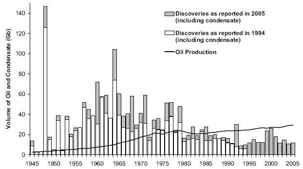
Figure 23: Discovery Data plotted with minimal filtering

Figure 24: Discovery Data with a 3-year moving average

Application of the Dispersive Discovery + Oil Shock Model to Global Production

In Figure 2, I overlaid a Dispersive Discovery fit to the data. In this section of the post, I explain the rational for the parameter selection and point out a flaw in my original assumption when I first tried to fit the Oil Shock Model a couple of years ago.

Jean Laherrere of ASPO France last year presented a paper entitled "Uncertainty on data and forecasts". A TOD commenter had pointed out the following figures from Pp.58 and 59:

Figure 25: World Crude Discovery Data

Figure 26: World Crude Discovery Data

I eventually put two and two together and realized that the NGL portion of the data really had little to do with typical crude oil discoveries; as finding oil only occasionally coincides with natural gas discoveries. Khebab has duly noted this as he always references the Shock Oil model with the caption "Crude Oil + NGL". Taking the hint, I refit the shock model to better represent the lower peak of crude-only production data. This essentially scales back the peak by about 10% as shown in the second figure above. I claim a mixture of ignorance and sloppy thinking for overlooking this rather clear error.

So I restarted with the assumption that the discoveries comprised only crude oil, and any NGL would come from separate natural gas discoveries. This meant that that I could use the same discovery model on discovery data, but needed to reduce the overcompensation on extraction rate to remove the "phantom" NGL production that crept into the oil shock production profile. This essentially will defer the peak because of the decreased extractive force on the discovered reserves.

I fit the discovery plot by Laherrere to the dispersive discovery model with a cumulative limit of 2800 GB and a cubic-quadratic rate of 0.01 (i.e n=6 for the power-law). This gives the blue line in Figure 27 below.

Figure 27: Discovery Data + Shock Model for World Crude

For the oil shock production model, I used {fallow,construction,maturation} rates of {0.167,0.125,0.1} to establish the stochastic latency between discovery and production. I tuned to match the shocks via the following extraction rate profile:

Figure 28: Shock profile associated with Fig.27

As a bottom-line, this estimate fits in between the original oil shock profile that I produced a couple of years ago and the more recent oil shock model that used a model of the perhaps more optimistic Shell discovery data from earlier this year. I now have confidence that the discovery data by Shell, which Khebab had crucially observed had the cryptic small print scale "boe" (i.e. barrels of oil equivalent), should probably better represent the total Crude Oil + NGL production profile. Thus, we have the following set of models that I alternately take blame for (the original mismatched model) and now dare to take credit for (the latter two).

Original Model(peak=2003) < No NGL(peak=2008) < Shell data of BOE(peak=2010)

I still find it endlessly fascinating how the peak position of the models do not show the huge sensitivity to changes that one would expect with the large differences in the underlying URR. When it comes down to it, shifts of a few years don't mean much in the greater scheme of things. However, how we conserve and transition on the backside will make all the difference in the world.

Production as Discovery?

In the comments section to the dispersive oil discovery model post, Khebab applied the equation to USA data. As the model should scale from global down to distinct regions, these kinds of analyses provide a good test to the validity of the model.

In particular, Khebab concentrated on the data near the peak position to ostensibly try to figure out the potential effects of reserve growth on reported discoveries. He generated a very interesting preliminary result which deserves careful consideration (if Khebab does not pursue this further, I definitely will). In any case, it definitely got me going to investigate data from some fresh perspectives. For one, I believe that the Dispersive Discovery model will prove useful for understanding reserve growth on individual reservoirs, as the uncertainty in explored volume plays in much the same way as it does on a larger scale. In fact I originally proposed a dispersion analysis on a much smaller scale (calling it Apparent Reserve Growth) before I applied it to USA and global discoveries.

As another example, after grinding away for awhile on the available USA production and discovery data, I noticed that over the larger range of USA discoveries, i.e. inferring from production back to 1859, the general profile for yearly discoveries would not affect the production profile that much on a semi-log plot. The shock model extraction model to first order shifts the discovery curve and broadens/scales the peak shape a bit -- something fairly well understood if you consider that the shock model acts like a phase-shifting IIR filter. So on a whim, and figuring that we may have a good empirical result, I tried fitting the USA production data to the dispersive discovery model, bypassing the shock model response.

I used the USA production data from EIA which extends back to 1859 and to the first recorded production out of Titusville, PA of 2000 barrels (see for historical time-line). I plotted this in Figure 29 on a semi-log plot to cover the substantial dynamic range in the data.

Figure 29: USA Production mapped as a pure Discovery Model

This curve used the n=6 equation, an initial t_0 of 1838, a value for k of 0.0000215 (in units of 1000 barrels to match EIA), and a D_d of 260 GB.

D(t) = kt⁶*(1-exp(-D_d/kt⁶))
dD(t)/dt = 6kt⁵*(1-exp(-D_d/kt⁶)*(1+D_d/kt⁶))

The peak appears right around 1971. I essentially set P(t) = dD(t)/dt as the model curve.

Figure 30: USA oil production early years

I find this result very intriguing because, with just a few parameters, we can effectively fit the range of oil production over 3 orders of magnitude, hit the peak position, produce an arguable t_0 (thanks Khebab for this insight), and actually generate a predictive down-slope for the out-years. Even the only point that doesn't fit on the curve, the initial year's data from Drake's well, figures somewhere in the ballpark considering this strike arose from a purely discrete and deterministic draw (see the Monte Carlo simulations above) from the larger context of a stochastic model. (I nicked Figure 30 off of an honors thesis, look at the date of the reference!)

Stuart Staniford of TOD originally tried to fit the USA curve on a semi-log plot, and had some arguable success with a Gaussian fit. Over the dynamic range, it fit much better than a logistic, but unfortunately did not nail the peak position and didn't appear to predict future production. The gaussian also did not make much sense apart from some hand-wavy central limit theorem considerations.

Even before Staniford, King Hubbert gave the semi-log fit a try and perhaps mistakenly saw an exponential increase in production from a portion of the curve -- something that I would consider a coincidental flat part in the power-law growth curve.

Figure 31: World Crude Discovery Data

---

Conclusions

The Dispersive Discovery model shows promise at describing:

1. Oil and NG discoveries as a function of cumulative depth.
2. Oil discoveries as a function of time through a power-law growth term.
   
3. Together with a Log-Normal size distribution, the statistical fluctuations in discoveries. We can easily represent the closed-form solution in terms of a Monte Carlo algorithm.
   
4. Together with the Oil Shock Model, global crude oil production.
5. Over a wide dynamic range, the overall production shape. Look at USA production in historical terms for a good example.
   
6. Reserve growth of individual reservoirs.
   

---

References

¹ "The Black Swan: The Impact of the Highly Improbable" by Nassim Nicholas Taleb. The discovery of a black swan occurred in Australia, which no one had really explored up to that point. The idea that huge numbers of large oil reservoirs could still get discovered presents an optical illusion of sorts. The unlikely possibility of a huge new find hasn't as much to do with intuition, as to do with the fact that we have probed much of the potential volume. And the maximum number number of finds occur at the peak of the dispersively swept volume. So the possibility of finding a Black Swan becomes more and more remote after we explore everything on earth.

² These same charts show up in an obscure Fishing Facts article dated 1976, where the magazine's editor decided to adapt the figures from a Senate committee hearing that Hubbert was invited to testify to.

Fig. 5 Average discoveries of crude oil per loot lor each 100 million feet of exploratory drilling in the U.S. 48 states and adjacent continental shelves. Adapted by Howard L. Baumann of Fishing Facts Magazine from Hubbert 1971 report to U.S. Senate Committee. "U.S. Energy Resources, A Review As Of 1972." Part I, A Background Paper prepared at the request of Henry M. Jackson, Chairman: Committee on Interior and Insular Affairs, United States Senate, June 1974.

Fig.6 Estimation of ultimate total crude oil production for the U.S. 48 states and adjacent continental shelves; by comparing actual discovery rates of crude oil per foot of exploratory drilling against the cumulative total footage of exploratory drilling. A comparison is also shown with the U.S. Geol. Survey (Zapp Hypothesis) estimate.

Like I said, this stuff is within arm's reach and has been, in fact, staring at us in the face for years.

³ I found a few references which said "The United States has proved gas reserves estimated (as of January 2005) at about 192 trillion cubic feet (tcf)" and from NETL this:

U.S. natural gas produced to date (990 Tcf) and proved reserves currently being targeted by producers (183 Tcf) are just the tip of resources in place. Vast technically recoverable resources exist -- estimated at 1,400 trillion cubic feet -- yet most are currently too expensive to produce. This category includes deep gas, tight gas in low permeability sandstone formations, coal bed natural gas, and gas shales. In addition, methane hydrates represent enormous future potential, estimated at 200,000 trillion cubic feet.

This together with the following reference indicate the current estimate of NG reserves lies between 1173 and 1190 TCF (Terra Cubic Foot = 10¹² ft³).

How much Natural Gas is there? Depletion Risk and Supply Security Modelling

US NG Technically Recoverable Resources   US NG Resources
(EIA, 1/1/2000, Trillion ft3)            (NPC, 1/1/1999, Trillion ft3)
---------------------------------------   -----------------------------
Non associated undiscovered gas 247.71    Old fields                305
Inferred reserves               232.70    New fields                847
Unconventional gas recovery     369.59    Unconventional            428
Associated-dissolved gas        140.89                
Alaskan gas                      32.32    Alaskan gas (old fields)   32
Proved reserves                 167.41    Proved reserves           167
Total Natural Gas              1190.62    Total Natural Gas        1779

⁴ I have an alternative MC algorithm here that takes a different approach and shortcuts a step.

Highlights of low-lifes

I haven't a clue how The Special Ed got invited to a Chevron and API (American Petroleum Institute) sponsored session on oil technology and energy policy.

API has underwritten Edward Morrissey’s travel expenses to attend the Chevron location tour in Houston and Corpus Christi, Texas. Edward is not required to blog about API initiatives. The only requirement as a condition of underwriting these expenses was to include this disclosure of this relationship on his blog.

Not that I would ever want to attend such a propaganda-filled event, but clearly the API and Chevron cherry-picked the slovenly right-wing blogosphere, primarily for their spectacular failure to report on anything related to the negative aspects of oil depletion. Even though Ed blogs at a diarrhea-ic rate daily (and he pops up a yakkity-yak audio feed to boot!), he and his cohorts have referenced peak oil rarely, the only significant time within the past month (10/22/2007) here:

It's nothing more than scaremongering, something at which the Peak Oil advocates excel.

Many different issues can cause production declines other than a reduction in the resource. War can impact production, as can political instability. One major producer, Iran, has significant economic sanctions against it that impacts their production capacity. Another producer, Venezuela, has conducted a nationalization policy that has also reduced its overall production. Producers that form cartels such as OPEC artificially set production levels for economic purposes, which renders these declines as analytically unreliable for purposes of determining resource availability.

It also doesn't account for the willful lack of production where known resources exist. That primarily applies to the US, where reserves exist on both coasts and in Alaska that we refuse to touch. We could deflate global oil prices and get more energy independence in the near- and mid-term simply by pumping our own crude. The US refuses to do so, however, for reasons of politics and not of potential supply.

Ed obviously did a bit of pimping to prepare for his fancy trip. After his special prom date he hasn't said much either, apart from some rather tepid live blogging. I don't claim to find anything new in making this observation, as his fellow bloggers at the Northern Axis Radio Network haven't mentioned peak oil much either. For example, I estimated that the fellow Axis-members, the Powerline bloggers never mentioned "peak oil" a few years ago, and still don't talk about it.

And the honorary member of the Axis, Hugh "Spew Spewitt" Hewitt of the larger encompassing ClownHall consortium had this exchange today during a long radio interview with propagandist Ahmed Chalabi when he claimed :

AC: I think Iraq is the only country in the world now that can actually produce 8 million barrels of oil a day from here until the end of the century. Iraq is rich. Iraq also has a very, very competent and smart population. We have high levels…(Call dropped)

- - (pop) - -

HH: Dr. Chalabi, when we got cut off, you were saying that Iraq is a rich country, capable of producing 8 million barrels of oil a day from now until the end of the century. What’s the implication of that for Iraq ten years from now, and for America’s role there? ..... (my emphasis since they rubbed it in)

Hewitt apparently accepted the claim in keeping with the prevailing right-wing attitudes, and the master salesman Chalabi closed the deal on the sucker.

After confronting this kind of blindered, blinkered attitude from the right daily, I tend to agree with the philosophy submitted by thereisnospoon at DailyKos. In a diary entitled "It's the Existential Threat to Conservatism, Stupid!", spoon uses arguments of the global warming denialists

the need to take anthropogenic climate change seriously is a threat to the entire premise of modern conservative thought--specifically regarding the deification of untrammelled free markets.

This essentially blends right into the oil depletion iceberg that similarly threatens the free-market Titanic.

I tend to think that the insular nature of the Northern Axis and Clown Hall membership also tends to create an incestuous spiral into like-minded thinking that, for me at least, raises some intriguing perspectives. In particular, the narrow insularity they exhibit lead me to the realization that the brain-trust of The Oil Drum has quite an open, and largely global, representation. Khebab, Euan Mearns, Stuart Staniford, Luís de Sousa, Rembrandt Koppelaar, and the TOD ownership and the spin-offs (with Big Gav hosting a down-under TOD), truly open up the discussion and prevents the blind acceptance of existential threats that the entire right-wing furtively prepare for while in their own patriotic clown huddle.

---

I guarantee a guest post to The Oil Drum before the end of the week. Khebab kindly notified me that an updated summary of the latest and greatest depletion modeling could prove useful. I'm tempted to title the post "Existential Threats: Proven Real, Deal With It".

Monte Carlo Algorithm for Dispersive Discoveries

You can derive the dispersive discovery curve quite easily, but I find it instructive as well to verify it via a Monte Carlo simulation.

The pseudo-code for the random number generation looks like the following (which uses the standard trick for inverting an exponential distribution):

for Depth in 1..Probing_Depth loop
 Amt_Discovered := 0.0;
 for I in 1..N loop -- reduces sampling noise
   Draw := Random (0.0 .. 1.0);
   Random_Depth := -Depth * Natural_Log (Draw);
   if Value > L0 then
     Amt_Discovered := L0 + Amt_Discovered;
   else
     Amt_Discovered := Random_Depth + Amt_Discovered;
   end if;
 end loop;
 -- Print Depth + Amt_Discovered/N
end loop;

The basic idea says that if you draw a depth deeper than L0 (the maximum depth for finding something), then cumulatively you can only pro-rate to L0. Otherwise, you will find discoveries proportional to the depth of the random variable probe, Random_Depth (or lambda below). This gives you an idea of how to do a stochastic integration. Remember, we only have an average idea of what probe depth we have, which gives us the dispersion on the amount discovered.

Gibson vs Eraser

Disturbingly difficult to
discern the difference.

---

On a related note, I have never seen a worse reputedly science-based blog than "Climate Audit". In fact, I find it so bad that the award it got for Best Science Blog immediately invalidates the lesser half of the blogosphere's contribution to science completely.


Update from comments: Gumby also upset about eraser family resemblance.


Another Update: Many of the climate change deniers have fallen for this hoax of epic proportions. In their (Rush Limbaugh, et al) desperate quest to find any evidence to grasp on to, they choose a well-done spoof. I just love the equation style the spoofers have chosen

Q²uct, yΦ³= ∑cy³42

or this one

4δ161 x Λ³Жญ5,6,1,8Φ-4 = {(ΣΨ²Њyt3 - 14๖P9) x 49}

2β x ⅜kxgt -§

That final character, which last time I checked, we usually use as a word processor flow marker takes the cake for incredulity. It basically screams, "You idiots, can't you see this is all gibberish?". But of course the Gibson crowd fall for it anyways (the slugs at Climate Audit apparently a bit too slow to catch on one way or the other). Because, of course, their stupidity knows no bounds, and the reservoir for new wing-nuts to join the Clown Hall circus remains infinite.

Dispersive Natural Gas Discoveries

As a follow-up to the last post on the Dispersive Discovery model, I decided to apply the same technique to US Natural Gas discoveries.

As background, I found a few references which said "The United States has proved gas reserves estimated (as of January 2005) at about 192 trillion cubic feet (tcf)" and from NETL this:

U.S. natural gas produced to date (990 Tcf) and proved reserves currently being targeted by producers (183 Tcf) are just the tip of resources in place. Vast technically recoverable resources exist -- estimated at 1,400 trillion cubic feet -- yet most are currently too expensive to produce. This category includes deep gas, tight gas in low permeability sandstone formations, coal bed natural gas, and gas shales. In addition, methane hydrates represent enormous future potential, estimated at 200,000 trillion cubic feet.

This together with the following reference indicate the current estimate of NG reserves lies between 1173 and 1190 TCF (Terra Cubic Foot = 10¹² ft³).

How much Natural Gas is there? Depletion Risk and Supply Security Modelling

US NG Technically Recoverable Resources   US NG Resources
(EIA, 1/1/2000, Trillion ft3)            (NPC, 1/1/1999, Trillion ft3)
---------------------------------------   -----------------------------
Non associated undiscovered gas 247.71    Old fields                305
Inferred reserves               232.70    New fields                847
Unconventional gas recovery     369.59    Unconventional            428
Associated-dissolved gas        140.89                 
Alaskan gas                      32.32    Alaskan gas (old fields)   32
Proved reserves                 167.41    Proved reserves           167
Total Natural Gas              1190.62    Total Natural Gas        1779

Hubbert originally plotted yearly discoveries per cumulative footage drilled for both oil and natural gas. I also found a curve for Natural Gas at this reference (may be the same one as found by McManus).

Interesting that if we fit the cumulative discovery data to the naive exponential that the curve matches very well on the upslope (see below) but that the asymptote arrives way too early, obviously missing all the dispersed discoveries covered by the alternative model. The dispersive discovery adds a good 20% extra reaching an asymptote of 1130, coming much closer to the value from NETL of 1190.

Although a bit unwieldy, one can linearize the dispersive discovery curves, similar to what oil analysts do with Hubbert Linearization. Although it swings wildly initially, I can easily see the linear agreement with a correlation coefficient very nearly one and a near zero extrapolated y-intercept.

As a comparison, I plotted the previously discussed fits for USA oil discoveries and found the same general agreement in linearization between NG and oil.

(note that the naive exponential that Hubbert used below overshoots the fit to better match the asymptote but still falls short of the alternative model's asymptote, and which also fits the bulk of the data points much better)


Every bit of data tends to corroborate that the dispersive discovery model works quite effectively in both providing an understanding on how we actually make discoveries in a reserve growth fashion and in mathematically describing the real data.

note: on some of the charts, the correlated fit does not show the decimal points in the linear equations due to a bug in the plotting program.