The Oil ConunDRUM

I synthesized the last several years of blog content and placed it into a book tentatively called The Oil ConunDRUM  (ultimately titled Mathematical Geoenergy published by Wiley/AGU in 2019). This document turned into a treatise of topics relating to the role of disorder and entropy in the applied sciences. Volume 1 is mainly on the analysis of the decline in global oil production, while Volume 2 uses often related analysis in studying renewable sources of energy and how entropy plays a role in our environment and everyday life.

This is a list of the novel areas of research, listed in what I consider a ranked order of originality:

1. The Oil Shock Model.
   A data flow model of oil extraction and production which allows for perturbations.
   
   
2. The Dispersive Discovery Model.
   A probabilistic model of resource discovery which accounts for technological advancement and a finite search volume.
   
   
3. The Reservoir Size Dispersive Aggregation Model.
   A first-principles model that explains and describes the size distribution of oil reservoirs and fields around the world.
   
   
4. Solving the Reserve Growth "enigma".
   An application of dispersive discovery on a localized level which models the hyperbolic reserve growth characteristics observed.
   
   
5. Shocklets.
   A kernel approach to characterizing production from individual fields.
   
   
6. Reserve Growth, Creaming Curve, and Size Distribution Linearization.
   An obvious linearization of this family of curves, related to HL but more useful since it stems from first principles.
   
   
7. The Hubbert Peak Logistic Curve explained.
   The Logistic curve is trivially explained by dispersive discovery with exponential technology advancement.
   
   
8. Laplace Transform Analysis of Dispersive Discovery.
   Dispersion curves are solved by looking up the Laplace transform of the spatial uncertainty profile.
   
   
9. The Maximum Entropy Principle and the Entropic Dispersion Framework.
   The generalized math framework applied to many models of disorder, natural or man-made. Explains the origin of the entroplet.
   
   
10. Gompertz Decline Model.
    Exponentially increasing extraction rates lead to steep production decline.
    
    
11. Anomalous Behavior in Dispersive Transport explained.
    Photovoltaic (PV) material made from disordered and amorphous semiconductor material shows poor photoresponse characteristics. Solution to simple entropic dispersion relations or the more general Fokker-Planck leads to good agreement with the data over orders of magnitude in current and response times.
    
    
12. Framework for understanding Breakthrough Curves and Solute Transport in Porous Materials.
    The same disordered Fokker-Planck construction explains the dispersive transport of solute in groundwater or liquids flowing in porous materials.
    
    
13. The Dynamics of Atmospheric CO2 buildup and extrapolation.
    Used the oil shock model to convolve a fat-tailed CO2 residence time impulse response function with a fossil-fuel stimulus. This shows the long latency of CO2 buildup very straightforwardly.
    
    
14. Terrain Slope Distribution Analysis.
    Explanation and derivation of the topographic slope distribution across the USA. This uses mean energy and maximum entropy principle.
    
    
15. Reliability Analysis and understanding the "bathtub curve".
    Using a dispersion in failure rates to generate the characteristic bathtub curves of failure occurrences in parts and components.
    
    
16. Wind Energy Analysis.
    Universality of wind energy probability distribution by applying maximum entropy to the mean energy observed. Data from Canada and Germany.
    
    
17. Dispersion Analysis of Human Transportation Statistics.
    Alternate take on the empirical distribution of travel times between geographical points. This uses a maximum entropy approximation to the mean speed and mean distance across all the data points.
    
    
18. The Overshoot Point (TOP) and the Oil Production Plateau.
    How increases in extraction rate can maintain production levels.
    
    
19. Analysis of Relative Species Abundance.
    Dispersive evolution of species according to Maximum Entropy Principle leads to characteristic distribution of species abundance.
    
    
20. Lake Size Distribution.
    Analogous to explaining reservoir size distribution, uses similar arguments to derive the distribution of freshwater lake sizes. This provides a good feel for how often super-giant reservoirs and Great Lakes occur (by comparison)
    
    
21. Labor Productivity Learning Curve Model.
    A simple relative productivity model based on uncertainty of a diminishing return learning curve gradient over a large labor pool (in this case Japan).
    
    
22. Project Scheduling and Bottlenecking.
    Explanation of how uncertainty in meeting project deadlines or task durations caused by a spread of productivity rates leads to probabilistic schedule slips with fat-tails. Answers why projects don't complete on time.
    
    
23. The Stochastic Model of Popcorn Popping.
    The novel explanation of why popcorn popping follows the same bell-shaped curve of the Hubbert Peak in oil production.
    
    
24. The Quandary of Infinite Reserves due to Fat-Tail Statistics.
    Demonstrated that even infinite reserves can lead to limited resource production in the face of maximum extraction constraints.
    
    
25. Oil Recovery Factor Model.
    A model of oil recovery which takes into account reservoir size.
    
    
26. Network Transit Time Statistics.
    Dispersion in TCP/IP transport rates leads to the measured fat-tails in round-trip time statistics on loaded networks.
    
    
27. Language Evolution Model.
    Model for relative language adoption which depends on critical mass of acceptance.
    
    
28. Web Link Growth Model.
    Model for relative popularity of web sites which follows a diminishing return learning curve model.
    
    
29. Scientific Citation Growth Model.
    Same model used for explaining scientific citation indexing growth.
    
    
30. Particle and Crystal Growth Statistics.
    Detailed model of ice crystal size distribution in high-altitude cirrus clouds.
    
    
31. Rainfall Amount Dispersion.
    Explanation of rainfall variation based on dispersion in rate of cloud build-up along with dispersion in critical size.
    
    
32. Earthquake Magnitude Distribution.
    Distribution of earthquake magnitudes based on dispersion of energy buildup and critical threshold.
    
    
33. Income Disparity Distribution.
    Relative income distribution which includes inflection point to to compounding interest growth on investments.
    
    
34. Insurance Payout Analysis, and Hyperbolic Discounting.
    Fat-tail analysis of risk and estimation.
    
    
35. Thermal Entropic Dispersion Analysis.
    Solving the Fokker-Planck equation or Fourier's Law for thermal diffusion in a disordered environment. A subtle effect.
    
    
36. GPS Acquisition Time Analysis.
    Engineering analysis of GPS cold-start acquisition times.
    

You can refer back to details in the blog, but The Oil ConunDRUM cleans everything up. It features quality mathematical markup, references to scholarly work, a full subject index, hypertext table of contents, several hundred figures with captions, footnotes and sidebars with editorial commentary, embedded historical documents, source code appendices, and tables of nomenclature and glossary.

---

EDIT (1/21/11): Here is a critique from TOD. I can only assume the commenter doesn't understand the concept of convolution or doesn't realize that such a useful technique exists:

Your methods are fundamentally flawed you cannot aggregate across producing basins like you do. Its simply wrong.
To add multiple producing basins together you must adjust the time variable such that all of them start production at the same time or if they have peaked all the peaks are aligned.
The time that a basin was discovered and put into production is an irrelevant random variable and has no influence on the ultimate URR.
If you don't correctly normalize the time variable across basins your work is simply garbage. There is no coupling between basins and no reason to average them based on real time. Its junk math. No simple function exists in real time to describe the aggregate production profile.
The US simply happened to have its larger basins developed about the same time in real time. Hubbert's original analysis worked simply because the error in the normalized time and real time was small.

One of the mysteries of science and mathematics is the role of entropy. The mathematician Gian-Carlo Rota from MIT had this to say just a few years ago:
The take on this is that as Rota says about the Maximum Entropy Principle "Among all mathematical recipes, this is to the best of my knowledge the one that has found the most striking applications in engineering practice", yet it retains this sense of mystery in that no one can really prove it -- entropy just IS and by its existence, you have to deal with it the best you can.

EDIT (1/31/11): In the book, the last prediction of global crude production I made was a while ago. Here is an update:


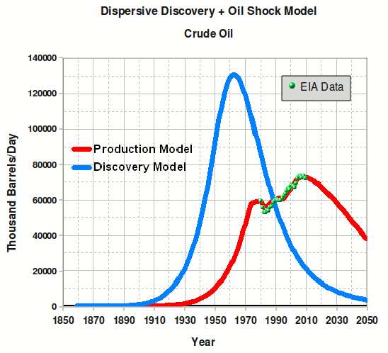
The chart above is the best guess model from 2007 using the combined Dispersive Discovery+Oil Shock Model for crude. Apart from a conversion from barrels/year to barrels/day, this is the same model as I used in a 2007 TOD post and documented in The Oil ConunDRUM. The recent data from EIA is shown as the green dots back to 1980. I always find it interesting to take the 10,000 foot view. What may look like a plateau up close, may actually be part of the curve at a distance.

EDIT (2/22/2011): An additional USA Shock Model not included in the book. I included Alaska in this model.

Discovery data transcribed from this figure; the discoveries seem to end in 1985, so I extended the data with a dispersive discovery model. I added in Alaska North Slope at 22 billion barrels in 1968 and a small 300 million barrel starter discovery in 1858.
.
The blue line in the Dispersive Discovery Model is this equation, which is essentially a scaled version of the world model:
DD(t)=(1-exp(-URR/(B*((t-t')^6))))*B*((t-t')^6), URR=240,000 million barrels, B=2E-7, t'=1835.

I did not include any perturbation shocks to keep it simple. Apart from the data, the following is the entirety of the Ruby code; the discovery.txt file is yearly discovery data, which is from the first graph. The second graph shows reserve.out and production.out.

cat discovery.txt | ruby exp.rb 0.07 | ruby exp.rb 0.07 | ruby exp.rb 0.07 > reserve.out
cat reserve.out | ruby exp.rb 0.08 >production.out

$ cat exp.rb

def exp(a, b)
rate = b
length = a.length
temp = 0.0
for i in 0..length do
output = (a[i].to_f + temp) * rate
temp = (a[i].to_f + temp) * (1.0 - rate)
puts output
end
end
exp(STDIN.readlines, ARGV[0].to_f)

Terrain Slopes

Entropy makes its mark everywhere. Take the case of modeling topography. How can we model and thus characterize disorder in the earth's terrain? Can we actually understand the extreme variability we see?

If we consider that immense forces cause upheaval in the crust then we can reason that the energy can also vary all over the map, so to speak. The process that transfers potential energy into kinetic energy to first order has to contain elements of randomness. To the huge internal forces within the earth, generating relief textures equates to a kind of brownian motion in relative terms -- over geological time, the terrain amounts to nothing more than inconsequential particles to the earth's powerful internal engine.

In a related sense the process also resembles the pressure distribution in the earth's atmosphere, a classic application of maximum entropy that we can re-apply in the case of modeling terrain slope distributions.

Premise. We take the terrain slope S as our random variable (defined as rise/run). The higher the slope, the more energetic the terrain. Applying Maximum Entropy to a section of terrain, we can approximate the local variations as a MaxEnt conditional probability density function:

p(S|E) = (1/cE) * exp(-S/cE)

where E is the local mean energy and c is a constant of proportionality. But we also assume that the mean E varies over a larger area that we are interested in, as in the superstatistical sense of applying a prior distribution.

p(E) = k*exp(-k*E)

where k is another MaxEnt measure of our uncertainty in the energy spread over a larger area.

The final probability is an integral over the marginal distribution consisting of the conditional multiplied by the prior:

p(S) = integral p(S|E) *p(E) dE from E=0 to infinity

This integrates as a BesselK function of the zero order, K₀, available on any spreadsheet program (see here for a similar derivation in an unrelated field).

p(S) = 2/S₀ * K₀(2*sqrt(S/S₀))

The average value of the terrain slope for this distribution is simply the value S₀.

Now we can try it on a large set of data. I downloaded all the DEM data for the 1 degree quadrangles (aka blocks/tiles) in the USA from the USGS web site. http://dds.cr.usgs.gov/pub/data/DEM/250/

This consists of post data at approximately 92 meter intervals (i.e. a fixed value of run) at 1:250,000 scale for the entire USA. I concentrated on the lower 48 and some spillover into Canada. I used curl to iteratively download each of the nearly 1000 quadrangle files on the server.

I then wrote a program to read the data from individual DEM files and calculate the slopes between adjacent posts and came up with an average slope (rise/run) of 0.039, approximately a 4% grade or 2.2 degrees pitch. I take the absolute values of all slopes so that the average is not zero.

The cumulative plot of terrain slopes for all 5 billion calculated slope points appears on the following chart (Figure 1). I also added the cumulative probability distribution of the BesselK model with the calculated average slope as the single adjustable parameter.

Figure 1: CDF of USA DEM data and the BesselK model with a small variation in S₀ (+/-4% about the average 0.037 rise/run) demonstrating sensitivity to the fit.

This kind of agreement does not just happen because of coincidence. It occurs because random forces contribute to maximizing the entropy of the topography. Enough variability exists for the terrain to reach an ergodic limit in filling the energy-constrained state space.

As supporting evidence, it turns out that we can generate a distribution that maps well to the prior by estimating the average slope from the conditional PDF of each of the 922 quadrangle blocks and then plotting this aggregate data set as another histogram (see Figure 2).

Figure 2: Generation of the prior distribution by taking the average slope of each of the nearly 1000 quadrangles . The best fit generates a value of S₀ (1/27=0.037) close to that used in Figure 1.

Practically speaking, we see the variability in slopes expressed at the two different levels. The entire USA at the integrated (BesselK model) level and the aggregated regions at the localized (exponential prior) level. These remain consistent as they agree on the single adjustable parameter S₀ .

The modeled distribution has many practical uses for analysis, including transportation studies and planning. Obviously, vehicles traveling up slopes use a significant amount of energy and you might like to have a model to base an analysis on without having to rely on the data by itself. (As a caveat, I did not include any of the spatial correlations that must also exist and might prove useful as well)

Perusing the recent research, I couldn't find anyone that had previously discovered this simple model. Not that they haven't tried, coming up with a good slope distribution model seems to amount to a mini Holy Grail among geophysicists. I went as far as dropping $10 to downloading the first paper, which turned out to be a bust.

1. Probabilistic description of topographic slope and aspect.
   G. Vico and A. Porporato, JOURNAL OF GEOPHYSICAL RESEARCH, VOL. 114, F01011, doi:10.1029/2008JF001038, 2009
   http://www.agu.org/journals/jf/jf0901/2008JF001038/2008JF001038.pdf
   
2. Nonlinear Processes in Geophysics Multifractal earth topography.
   J.-S. Gagnon, S. Lovejoy, and D. Schertzer, Nonlin. Processes Geophys., 13, 541–570, 2006
   http://hal.archives-ouvertes.fr/docs/00/33/10/93/PDF/npg-13-541-2006.pdf
   
3. PROPAGATION OF DEM UNCERTAINTY: AN INTERVAL ARITHMETIC APPROACH.
   G Gonçalves, XXII International Cartographic Conference, 2005
   http://www.cartesia.org/geodoc/icc2005/pdf/oral/TEMA7/Session%202/GIL%20GON%C7ALVES.pdf
4. SAR interferometry and statistical topography.
   Guarnieri, A.M. IEEE Transactions on Geoscience and Remote Sensing, Dec 2002
   http://home.dei.polimi.it/monti/papers/montiguarnieri02.pdf

If someone wants to generate Monte Carlo statistics for the BesselK model without having to do the probability inversion, the algorithm turns out surprisingly simple. Draw two independent random samples from a uniform [0.0 .. 1.0] interval, apply the natural log to each, multiply them together, and then multiply by the S₀ scaling constant. That will give the following cumulative if done 5 billion times, which is the same size as my USA DEM data sample.

Figure 3: Generation of the BesselK model via Monte Carlo.

The only statistical noise is at the 1e-9 level, same as in the DEM data.

Examples of some random-walk realizations drawing from a two-level model follow. The flatter regions occur more often reflecting the regional data.