Finding needles in a haystack

Cross-posted to The Oil Drum thanks to Khebab and The Editors

In school, we used to do horrendously difficult mathematical "word" problems routinely. I remember occasionally getting one right, but more often ended up punting on the problem, and then waiting for the teacher to explain the solution in all its elegant simplicity. Of course, just about every real-world problem contains inherent ambiguities and incomplete information. So we rarely get to see the elegant solution in our day-to-day work life. Sometimes we get lucky and nail a problem, but in the majority of cases, we eventually resort to creating a limited model of the problem domain and deal with that.

The problem that I have recently wrestled with has to do with predicting future oil discoveries based on historical dynamics. Ideally, I want to reduce it to a solution that has the elegance of a word problem, and not have to deal with messy economic and geologic factors that would quickly turn it into a rat's nest of complexity. Call me an optimist in this regard, but my intuition tells me that the solution remains as simple as ... finding needles in a haystack.

Simple as finding a needle in a haystack? Perhaps not so in regard to the actual process, but simple as in the premise behind the problem. Let me explain why this provides a good primer to the oil discovery problem. Scaled back to relative terms, the ratio of needles to hay compares intuitively to the ratio of oil to the earth's crust. So first and foremost, this rather naive analogy allows us to get our arms around a problem with just enough initial insight to get started-- the description of which amounts to nothing more than imagining that the haystack acts like the earth's crust and the needles serve as the pockets of oil. Statistically speaking, happening across a random needle in a haystack has a lot in common with running across a pocket of oil. We can also add technology and human incentive to the mix to extend the simple analogy before we migrate to the real problem.

So I present a starter word problem:

Given a large number of needles dispersed in a random spatial manner throughout a good-sized haystack, at what point in time would we find the maximum number of needles? As a nod to technology we get to monotonically increase our search efficiency as we dig through the stack, and we can add human helpers as we progress.

Answer: Obvious, and we don't have to even lift a pen. On average, the maximum discovery of needles occurs as we sift through the last of the volume, and once finished, the discovery rate drops to nil. So the instantaneous "discovery" rate looks similar to the curve at the right. The acceleration upward in the curve occurs as we get more proficient over time and can attract some help. Note that if we mixed larger nails and smaller pins with the needles and instead measured total weight or volume instead of quantity, we would have the same curve (this has implications for the oil discovery problem).

Next, let's make the word problem a bit more sophisticated. Say that instead of dispersing the needles randomly through the entire haystack, we only do it to a certain depth, and to top it off, we do not reveal to the needle and pin searchers this depth. They basically have to oversample the haystack to find all the needles. If you look at the following figure, we separate out the "easy" part of the search from the "difficult" part (i.e. difficult as in not finding much even though we expend the effort). The boxes represent monotonically increasing sampling volumes, which we use to sweep out the volume of the haystack.



Hand-Wavy Answer: Suffice to say, if we search top to bottom, we will similiarly reach a peak, but the peak will also contain a gradual backside. Intuitively, we can sense that the sharpness of the peak reduces as the sampling volume overlaps the region that contains the needles with the region absent of needles. And then as the sampling volume drifts even deeper, the amount discovered drops closer and closer to zero.

For us to draw the peak as a smooth curve, we need to add stochastic behavior to the search process. This can occur, for example, if the individual searchers have varying skills.

a stochastic variable is neither completely determined nor completely random; in other words, it contains an element of probability. A system containing one or more stochastic variables is probabilistically determined.

What really makes the haystack problem different than the global oil discovery doesn't lie in the basic word problem but rather in the application of randomness or dispersion to the problem. We have much greater uncertainties in the stochastic variables in the oil discovery problem, ranging from the uncertainty in the spread of search volumes to the spread in the amount of people/corporations involved in the search itself. We don't just deal with a single haystack, but multiple haystacks all over the world. So the sharply defined geometric discovery profile shown to the right gets washed out as a result of the statistical mechanics of the oil industry ant-people hard at work.

Final Exam Answer: Let's jump from haystacks to oil discovery. We solve the problem by making the generally useful assumption that the current swept volume search has an estimated mean, and a variance equal to the square of the mean. In other words, in the absence of having any knowledge in the distribution of instantaneous swept volumes, we assume a maximum entropy estimator and set the standard deviation to the mean. A damped exponential probability density function follows this constraint with the least amount of bias, maximum uncertainty, and a finite bound (the latter factor would rule out something like a log-normal distribution). The following curve demonstrates how the spread in values gets expressed in terms of error bars.

In a nutshell, we want to solve the discovery success rate of a swept volume realizing that part of the volume straddles empty space. In other words, to account for the effects of the dispersion of oversampled volume, we have to integrate the exponential probability density function (PDF) of volume over all of space, and determine the expected value of the cross-section. To solve the problem by baby-steps, we first take a look at the one-dimensional version of the problem, then extend it to three-dimensions, and finally add the time variation.

I originally used the following single-dimension equation derivation to solve the reserve growth "enigma" of a single reservoir.

In the three-dimensional case, the stochastic variable lambda represents current mean swept volume, the term x integrates over all volumes, and L₀ represents the finite container volume V_d. The outcome L-bar represents a kind of pro-rated proportion of discoveries made for the dispersed swept volume at a particular point in time.

By itself, the function corresponding to L-bar doesn't look like anything special, and indeed looks a lot like the cumulative of the exponential PDF. However, the fact that lambda monotonically increases with time, together with L-bar appearing in the denominator, gives it interesting temporal dynamics, of which I contend follows the empirical observations of cumulative oil discovery and that of reserve growth as well.

From first principles, we would expect that swept volume growth approaches a power-law, and likely a higher-order law. For example, considering the "gold-rush" attraction of prospecting resources alone, we would expect that linear growths in (a) oil exploration companies, (b) employees per company, and (c) technological improvements would likely contribute at least a quadratic law.^[1] In terms of the bottom-line, multiplying two linear growth rates generates a quadratic growth^[2], and multiplying more linear rates leads to higher order growth laws. As an example, you can see this power-law increase play out as evidenced by the historical increase in average oil well depth over the years (see ^[3] for data point references).

But of course, this only accounts for one dimension in the sampling volume. So if we make the assumption that the effective horizontal radius of the probe also increases with a quadratic law, we end up with a power-law order of n=2*3=6, where the 3 refers to number of dimensions in a volume. Because we actually use cumulative volume in the stochastic derivation, the order becomes 6 in the result shown below. When we make an assumption that the parameter k denotes a fraction of the swept volume that results in a cumulative discovery D(t), we can replace V_d with D_d, where D_d is essentially equivalent to a URR for discoveries.

D(t) = kt⁶*(1-exp(-D_d/kt⁶))

and the derivative of this for instantaneous discoveries (e.g. yearly discoveries) results in:

dD(t)/dt = 6kt⁵*(1-exp(-D_d/kt⁶)*(1+D_d/kt⁶))

For a family of power-law growth functions, the trend looks like the following set of curves. The salient point to note relates to how we trend toward an asymptotic limit at the volume V_d as the power-law index gets larger.


To briefly summarize how dispersion of prospecting effort affects the discovery process, consider the curve below. Initially, as the sampling probe stays well within the V_d limit, the dispersed mean comes out as expected since we do not oversample the volume. However, as the standard deviation excursions of the cumulative volume starts to bleed past V_d, the two curves start to diverge and a rounded discovery peak results.


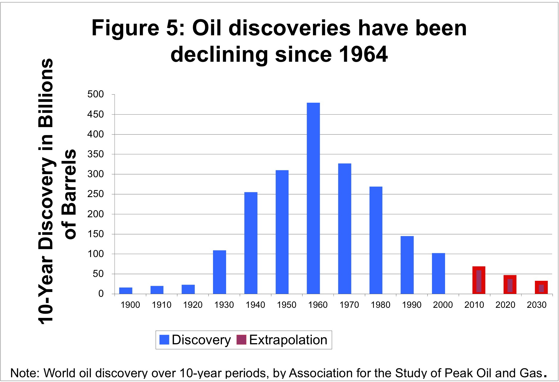
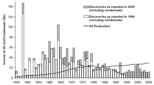
Scores of depletion analysts, including Laherrere, have pointed out the similarity of yearly discovery curves to the classic Hubbert curve itself. For the following discovery curve from Shell Oil (courtesy of a TOD post from Rembrandt) one can see the same general trend, albeit buried in the noisy fluctuations of yearly discoveries.

To remove the noise, we can generate a cumulative discovery curve. Apart from missing out on the cumulative data from the years post-1858 to the initial year of collected data, we can generate a good fit to the curve with an n=6 power-law dispersive growth function. (Note that the curve has a constraint to start in 1858, i.e. t=0, the "official" date which signalled the beginning of serious oil exploration)




Applying this modelled discovery curve to the Oil Shock production model (see the m o b j blog and a review by Khebab here at TOD), we come up with the following production extrapolation.

The oil shock parameters include a fallow latency of 6 years, a construction latency of 8 years, and a maturation latency of 10 years. It also includes the following extraction rate shock profile.

Interesting that this gives a production peak around the year 2010, even though the effective URR from the Shell discovery data amounts to 3.5 trillion barrels -- much higher than the lowball 2+ trillion estimate commonly bandied about by pessimistic peak oil analysts (note that the shell estimates uses the somewhat ambiguous "barrels of oil equivalent").

We can further substantiate the discovery fit by applying it to the USA data subset. For instance, let's consider what would happen if we used the same parameters from the global data to estimate U.S. discoveries. Note that the same constants (i.e. k and n=6) are used, but we change the D_d to reflect a fractional area of the US in comparison to the world.

World Land Area = 150,000,000.0 km²
USA Land Area = 10,000,000.0 km²

So to first-order, the D_d for USA is 1/15th that of the world's D_d (Roland Watson posted a similar sanity check recently on TOD with reference to USA and world URR). The following figure lays the cubic-quadratic discovery curve on top of Laherrere's data.

Within an order-of-magnitude, the fit doesn't look out-of-place. In the context of swept volume, it means that the USA reached its limit of easily discovered oil quicker than the rest of the world, which makes sense as serious oil exploration started in the USA.

---

After the equations have been solved, the result can be translated back into the ordinary language.

---

As far as word problems go, I don't consider the discovery model solution difficult in terms of the basic math. Perhaps we lack only an intuitive sense of how probabilities fit into the model. From one perspective, the uncertainty we have of the swept volume in relation to the finite volume of oil-bearing reservoirs reflects in our uncertainty with respect to reserve growth. In fact, I originally came up with this discovery model to understand the dynamics of reserve growth in a single reservoir and found that it has applicability to the larger global dynamics. Remember, that the estimated discoveries themselves have uncertainties built into them and only become solidified with the passage of time. As shown in the model derivation figure, the "depth of confidence" lambda term represents a real uncertainty of how much volume we have actually swept out. Only after oversampling the volumes do we sufficiently increase our confidence of our original estimate. Analysts typically use backdating to update earlier conservative estimates; in a way, we build backdating into the model by smearing out the estimate. Note that the roles of backdating discoveries and the maturation phase in the Oil Shock production model have a symbiotic relationship; if we have to deal with backdated data then the maturation phase takes longer and if we don't get backdated data, then the maturation gets reflected by delta discoveries that extend over time. To address this detail, Khebab believes that a Hybrid Shock Model has potential.

As far as other criticisms, I suppose one could question the actual relevance of a power-law growth as a driving function. In fact the formulation described here supports other growth laws, including monotonically increasing exponential growth. Furthermore, one could question whether we can sustain a power-law growth in the future, which together with extraction rate extrapolations, will have a significant impact on how future production will conceivably pan out. And to account for any further reserve growth, the fact that much of the fit curve occurs before the peak happens means that past discovery estimates have had a chance to mature and we have more confidence in the discovery decline profile. In my opinion, this makes it a fairly conservative estimator -- to substantiate this take a look at the huge effective URR for the Shell discovery data, which in all likelihood includes reserve growth, and note how it only impacts the peak date a few years from my previous shock model prediction of 2004 (which had no extrapolated future discovery data and used solely Laherrere's discovery data which had a much lower effective URR of around 2000 GBls).

Or, one could question the impact of super-giant discoveries on the smoothened discovery plot. Statistically, super-giants get treated like anything else in this model and they populate the volume with the same randomness. Predictably, one could also question the absence of deep geologic or economic considerations in the model. The canned response to that line of questioning is second nature to a seasoned statistical mechanic: physicists and other scientists apply such stochastic approximations all the time without a lot of fundamental problems. Why should this stochastic model become an exception to the rule?

I also have not opened up the future possibility of a levelling out or even general decline in discovery search effort. I gave this some serious effort in past blog postings, but realized that this would give too pessimistic a prediction and perhaps too much of an artificial constraint.

Finally, one could question why no one else in the oil industry thinks in terms of this kind of discovery model, in other words, why hasn't someone else found this proverbial needle in a haystack? Don't ask me; for all I know, an analyst in some energy corporation's back room has come up with the same idea and it has transformed into filing-cabinet intellectual property with no hope of seeing the light of day (i.e. what good would it do them financially?). Or perhaps, a similar idea remains buried in some academic journal, for which I lack the resources to discover on my own. But if my approach indeed has some originality and correctness to it, I can rationalize this with a more mundane explanation that comes from, in part, my experiences in solving problems in the research and software world. Occam says to rely on the simplest explanation to a problem; but what happens when two sufficiently separate but equally fundamental explanations contribute to a greater understanding? In these cases, we have to overcome the inertia of conventional wisdom.

To explain this rather philosophical point, I consider an oil depletion model as a two-stage word problem. The first part of the word problem relates to production (illustrated by the Oil Shock model) and the second part provides a model of the discovery input used to feed production (i.e. the basis of the Cubic-Quadratic discovery model desribed in this post). The relationship of two interacting models has some similarity to an aspect of software debugging instanced by the occasional defect that takes enormous resources to resolve. Or resembles in some ways to the laboratory anomaly that no one can pin down precisely by experiment. Invariably, the most difficult bugs to resolve result from two or more interacting defects. In my opinion, these remain the most elusive problems to solve simply because you don't normally think that more than one fundamental issue contributes to the cause of a root problem. And there you have an example of a real-world word problem. While everyone and their cousin wants to figure out oil depletion with a single freakin' logistic curve (excepting R²), as though that contains THE key to the kingdom, we realize that oil depletion may have two underlying forces at work -- namely, the discovery process followed by the extraction process. And so we rely on the wisdom of a divide-and-conquer strategy -- figure out the extraction/production problem all the while knowing that the discovery problem lays in waiting, or vice-versa. Now think back to the original "needle in the haystack" problem; notice that in that case, discovery and extraction occur at the same time. Once you find the needle you can extract it. But not so with oil, as discovery only starts the process that culminates in extraction and production. In my opinion, when we can understand the two problems individually, we can then solve the penultimate word problem of our times.

---

^[1] Note that parabolic growth is not the same as quadratic growth. Due to some historic conventions inherited from Silicon Valley, parabolic growth actually follows a fractional power-law growth, more precisely a square-root of time dependence.

^[2] See growth in wiki words for another real-world example of quadratic growth that occurs as we speak.

^[3] I gathered the max depth well chart from these sources: 1, 2, 3, 4, 5, 6, 7, 8, 9, 10

The Climate Change Nut-Case

I witnessed one of the most idiotic pieces of local journalism ever broadcast this evening on the ABC affiliate KSTP-TV. Better known for doing news stories about tobacco stores on fire and amusement rides gone terribly wrong, the news team at KSTP decided to do a local angle on global warming.

... so we pulled together a team of experts ...

Watching the hour-long show, The Climate Change Case, I saw the skeptical morons Christie, Ball, Lindzen, and Michaels featured prominently and the local weatherdork Dave Dahl fawn over some other wingnut in an interview.

All so pretentious and the more so because they deem themselves so important to preempt some prime-time crap because they seem to think they have earned their credentials by constantly showing us the latest murder-suicide that apparently someone else considers necessary to function in their day-to-day life.

I predict next, The Cost of Gas Case.

Filibuster

"Faced with the choice between changing one's mind and proving that there is no need to do so," said John Kenneth Galbraith, "almost everyone gets busy on the proof." --- via prospect

This quote cuts close to home, and cuts both ways.

The Republicans have a perpetual motion machine in the filibuster. John Kerry responded.

Monkeygrinder and Big Gav discover this simple but telling editorial cartoon.

In the more-fun-with-proofs category, Khebab has another installment at TOD of his periodic production forecast reviews.

Discovery Curves

This from a recent "quiz" post on TOD:


This resurrected from a Rembrandt K post on TOD:



And this from a Khebab post on TOD:


And finally the classic reference profile:






The differences between these curves result primarily from different amounts of filtering. The top one appears to sum up cumulative in each decade, resulting in a more-or-less symmetric bias. However the second has a fairly severe lagged moving average, resulting in the discovery peak shifting right quite a bit. The third shows little by way of filtering and includes superimposed backdating results. The fourth has a 3-year moving average, which I believe came from the unfiltered fifth curve due to Laherrere. I haven't found where I dug up the last curve from.

I figure instead of filtering the data via moving averages, it might make more sense to combine discovery data from different sources and use that as a noise reduction/averaging technique. Ideally I would also like to use a cumulative but that suffers a bit from not having any pre-1900 discovery data.

Lotka-Volterra equation

A poster at peakoil.com, jimk, tried his hand at modifying the Logistic equation model describing oil depletion dynamics. He made a decent attempt at correcting what I always claimed as a weak spot of the Logistic model: that the Logistic formulation needs a "biological" entity to propagate exponential growth but that nothing in its derivation hints at this fundamental requirement. So, jimk made an interesting substitution as shown below:

As it turns out, his modified equation pretty much matches the Lotka-Volterra equation which biologists use to model quasi-cyclic oscillations of "renewable" resources such as foxes and rabbits as well as other "predator-prey" relationships.


So, in jimk's equations R = population of prey and P = population of predators. R starts at some value and decays nonlinearly and proportionally to how much prey remains and how many predators exist to eat them. Similarly, the predator P starts at some value and grows proportionally to how many predators exist and how much prey exist (i.e. exponential birth rate sped up by food supply). The predator population also dies in proportion to its current population (i.e. classical death rate).

P : P*R
This only differs from the conventional L-V in that the prey does not have its own birth rate. So it generates a "non-renewable" variant of the L-V solution.

Humans = P = the predators
Oil = R = the prey

Interesting analogy, but as commenter Doly said at the peakoil.com thread:

I can see a certain logic in the way the equations are tweaked to show the economic incentives to extract oil, but it's still an oversimplified picture of the economy. And of course, there's nothing there to indicate geological constraints, which really should be there.

I agree, that the lack of geological constraints makes the rise and fall of the modified L-V equations depend solely on the non-linear interaction between the rates of change of the two populations. In effect, just as in the logistic model, the parameters have no physical meaning with respect to oil depletion. Plus, we can only solve this set of equations numerically -- which makes it hard to come up with a URR. The fact that the Logistic equation happens to generate an analytical URR and that the modified L-V doesn't means that the Logistic just got lucky. Convenience and expediency for the Logistic win out over a slightly more principled construction in the case of the L-V formulation.

But if we want a real geological constraint, the discovery/shock model remains the one to beat.

Update: I probably should take back the assertion I made regarding the difficulty in estimating the URR for the L-V equations. Even though I haven't verified it through the computational wringer, I suspect that the URR corresponds to the initial value for R(0) (i.e. R(t) at time=0).

Mars Sea of Oil

Weird Theory