
Hydrogeology for Dummies
A running theme of this blog involves the reduction of seemingly complex behaviors into simple mathematical formulations. It remains a bit of a mystery to me why in many situations that no one has either (a) done this work on their own or (b) uncovered the work of someone else who has done the simplifying analysis years ago.
The majority of scientists practicing mainstream research have furthered the cause by following the lead of others who go down blind alleys and over-complicate the analysis. I suspect that a few complicate matters intentionally, as it demonstrates to other scientists their intellectual prowess. In certain cases, creating a private world of intricate analysis acts as a kind of moat around which they can fortify their specialty discipline.
Of course, this doesn't happen universally. Certainly we run across many scientific and engineering subdisciplines that have gone through years of scrubbing. In these cases, the most salient and simple analyses have emerged and stood the test of time. They often share the same traits of elegance and crystalline transparency so that we can use their patterns to understand the world without a lot of extra effort. To me, that seems a reasonable goal to strive for.
In this post, I will go through the derivation of what I consider a very overlooked and simple argument having to do with the transport of materials in porous media -- much as what you would find in tracing a contaminant though a groundwater basin. Or what may happen if you frac for natural gas and open up new pathways to a drinking water aquifer. Or how oil will migrate to a reservoir over time, feeding the production output of a stripper well for years. Or what happens if you spill oil in a waterway.
Unfortunately, when you pose this kind of problem to a research geologist or hydrologist, you will have to prepare for an onslaught of ornate misdirection. They will either derive some hideous numerical model or possibly run a piece of commercial software. Apparently, they will never resort to plain logic and elementary first-principles considerations.
The Problem
1. Consider a contaminant that enters an aquifer in a single dose
2. Predict how long it will take to pass by a downstream location
3. How do you solve this problem?
A large scale experiment typically looks like this scenario:

 As a main premise, I assume that disorder plays a big role in providing a variety of pathways from source to sink. One can imagine that some paths might occur on the main waterway, providing a maximum speed or path of least resistance. Other paths may follow obstructions or diversions which will either slow down or speed up the flow from the main path.
 Figure 1: MaxEnt velocity distribution for absolute mean deviation
The calculation of downstream concentration, n(x,t), drops out of the Fokker-Planck equation if we ignore diffusion. Note the delta function, δ(x-vt), which describes a traveling pulse for each velocity component.
n(x,t) = ∫ p(v) δ(x-vt) dvNext we apply the Maximum Entropy Principle to generate a velocity distribution as shown in the Figure 1:
p(v) = 1/vm exp(-|v-vo|/vm)No other distribution has a higher entropy given that mean and an absolute deviation from the mean, so it ranks as the least biased estimator for that set of constraints. (Note that this does not describe the normal or Gaussian distribution as that requires a second-moment, i.e variance, constraint. It turns out that the mean deviation distribution, also known as the Laplace, is actually a smeared Gaussian where we have MaxEnt uncertainty in σ-squared. So Laplace entropy is higher than the Gaussian entropy)
We can trivially solve the integral to generate a concentration at some downstream location x (forget about adding extra dimensions as a one-dimensional result should suffice).
n(x,t) = 1/(vmt) exp(-|x/(vmt)-v0/vm|)Let's see how this works in practice.
I pulled data from a pair of papers from 2008, "Non-Fickian dispersion in porous media", T Le Borgne, P Gouze, et al. The scientists created a carefully controlled experiment, which relied on a customized apparatus for making precise measurements of the contaminant, a flourescent dye called uranine. The value of this particular experiment lies in the large dynamic range of the resultant data. The concentration runs over 4-orders of magnitude and the time scale 2-orders. Their own model, although generating a good fit to the data, needed a numerical calculation to solve, violating my assertion that we can model via simpler mechanisms.
The following figure allows for the wide dynamic range by plotting the concentration (also known as a breakthrough curve) on a log-log scale. The red triangles ◊ fit the Maximum Entropy dispersion model, n(x,t), for a fixed value of x and a value of vm/v0 = 0.18. By inverting the concentration we can get the probability distribution of velocities in the bottom figure; on a semi-log plot a symmetric two-sided exponential looks like a perfect isosceles triangle. Based on the outstanding fit and symmetric distribution I find it blatantly obvious that entropic mechanisms generate the dispersion observed. You won't get this parsimonious a fit from such a simple model -- with essentially a single parameter vm/v0 -- unless it has some real merit.
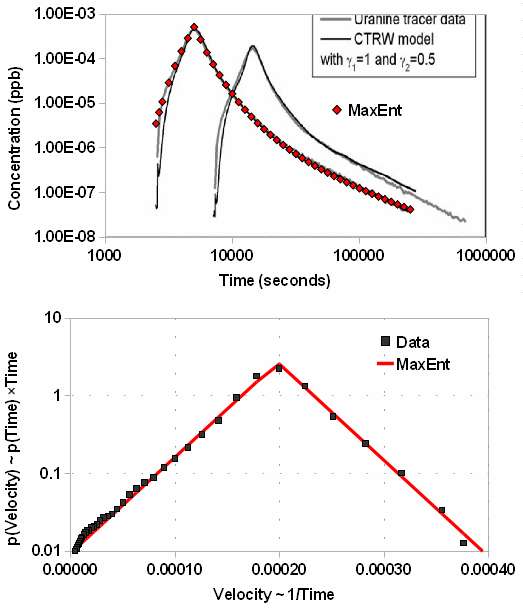 Figure 2: Breakthrough curve (top) and
measured velocity distribution (bottom)
for flourescent dye tracer experiment.
The simplicity of the model also points out how readily fat-tail effects emerge from entropic disorder. The power law drop-off obeys a 1/time behavior that certainly has consequences in terms of how long a contaminant will remain in a groundwater basin. Velocity dispersion with a mean MaxEnt constraint will always lead to a power-law drop-off in time (see more here).
See also these posts:
- http://mobjectivist.blogspot.com/2009/06/dispersive-transport.html
- http://mobjectivist.blogspot.com/2010/05/characterizing-mobility-in-disordered.html
- http://mobjectivist.blogspot.com/2010/05/fokker-planck-for-disordered-systems.html
posted by @whut at September 06, 2010
![]()
![]()


6 Comments:
Thanks again WHT. The simplicity and straightforward presentation of this post caused me to to review several Wikipedia pages on Maximum Entropy and the Fokker-Planck equation.
It's been a long time since I actually did the math for my graduate classes in quantum and statistical mechanics but I can still at least appreciate the approach.
I am pleased to know more about a statistical approach that minimizes assumptions and better models the data from our highly entropic real world.
If there were an Occam's Razor Award I would nominate you.
Cheers,
Jon
Thanks. I actually worked out the full Fokker-Planck for this case independently varying the diffusivity and mobility, but found that it didn't make much of a difference to the simple solution.
Fixed a bad link too.
It might be interesting at some point to team up and create an interactive modeling web page that allowed folks to tweak some of the input parameters in your statistical models (e.g. shock model) and immediately see the results, presumably plotted against real data.
My databrowser pages are all built with python and R so I'm sure we could find some common ground.
I have a version of the Shock Model witten in Python.
I'm an MSc hydrogeology student and was really struck by your post, I've never seen a similar approach considered before. My experience of hydrogeological models is that they're similar to climate models - everyone involved is always striving to maximise the complexity (with positive intentions though!). I struggled through your maths but can really appreciate the sense of simplicity here.
The result relies on having a decent estimate for Vm/Vo though, right? Surely that's in itself is something that would require quite complicated methods to predict? It would have to account for sorption, retardation, dispersivity etc.
I was just wondering if you had any thoughts on estimating the velocity ratio, and how that could be simplified?
Off to read through more of your archive now...
The Vm/V0 factor is essentially a guess as to the significance of the drift component and how much disorder you will anticipate seeing. Maximum entropy is subject to constraints but these constraints may only be known after taking some measurements.
A much more thorough explanation in my book The Oil ConunDrum
Post a Comment
<< Home