
Fokker-Planck for Disordered Systems
To get the cost of photovoltaic (PV) systems down, we will have to learn how to efficiently use crappy materials. By crap I mean that mass-produced PV materials will end up getting rolled or extruded or organically grown. Unless we perfect the process, most everything will turn out non-optimal. We already know the difference between clean-room cultivated single crystal semiconducting material and the defect-ridden and often amorphous materials that nature and entropy drives us to. For performance sensitive applications such as communications and computing we would only rarely consider disordered material as a candidate semiconductor. Certainly, the performance of these materials makes them unlikely candidates for high speed processing -- yet for solar cell applications, they may serve us well. In the end, we just have to learn how to understand and deal with crap.
The following will revisit a couple of previous posts where I outlined a novel way to analyze the behavior of disordered semiconducting material. I know for certain that no one has proposed the particular approach before. If it does exist, I certainly can't find it in the literature. From one perspective, this analysis sets forth a baseline for the characterization of a maximally disordered semiconductor.
Background
The prehistoric 1949 Haynes-Shockley experiment first measured the dynamic behavior of charged carriers in a semiconducting sample. It basically confirmed the solution of the diffusion (Fokker-Planck) equation and it demonstrated diffusion, drift, and recombination in a conceptually simple setup. This animated site gives a very interesting overview of PV electrical behavior.

Figure 1: Apparatus for the Haynes-Shockley experiment
This setup works according to theory for an ordered semiconductor with uniform properties but apparently gets a bit unwieldy for any disordered or non-uniform material sample. I inferred this as conventional wisdom since most scientists either punt or use heuristics partially derived from the inscrutable work of a select group of random-walk theorists (see Scher & Montroll).
I had previously applied a very straightforward interpretation to the problem of carrier transport in disordered material. My dispersion analysis essentially set aside the Fokker-Planck formalism for a mean value approximation where I tactically applied the Maximum Entropy Principle. In particular, I really like the MaxEnt solution because I can recite the solution from memory. It matches intuition in a conceptually simple way once you get into a disordered mind-set.
In the real Haynes-Shockley experiment, a pulse gets injected at one electrode, and a nearly pure time-of-flight (TOF) profile results. The initial pulse ends up spreading out in width a bit, but the detected pulse usually maintains the essential Gaussian sigmoid shape.
Adding Disorder
For the time-of-flight for a disordered system, the Maximum Entropy solution looks like:
q(t) = Q * exp(-w/(sqrt((μEt)2 + 2Dt))This essentially states that the expected amount of charge accumulated at one end of the sample (at a distance w) at time t, follows a maximum entropy probability distribution. The varying rates described by μ and D disperse the speed of the carriers so that a broadened profile results from the initial pulse spike.

The equation above formed the baseline for the interpretation I described initially here.
For completeness, I figured to test my luck and see if I can bull my way through the basic diffusion laws. If I could produce an equivalent solution by applying the Maximum Entropy Principle directly to the Fokker-Planck equation, then this would give a better foundation for the "inspection" result above.
The F-P diffusion equation gets expressed as a partial differential equation with a conservation law constraint:
 In this case D1=μ* (carrier mobility) and D2=D* (diffusion coefficient), and f(x,t)=n(x,t) (carrier concentration). With recombination, the solution in one-dimension looks like:
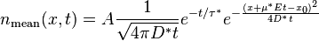 This of course works for well-ordered semiconductors, but D* and μ* will likely vary for disordered material. I made the standard substitution via the Einstein Relation for
D* = Vt μ*
From the basic physics, we can generate a maximum entropy density function for D
p(D*) = 1/D * exp(-D*/D)then
n(x,t) = Integral p(D*) * nmean(x,t) over all D*This looks hairy but the integral comes out straightforwardly as (ignoring the constant factors)
n(x,t) = 1/sqrt(t*(4D+t*(Eμ)2)) * exp(-x*R(t)) / R(t)where
R(t) = sqrt(1/(Dt) + E/(2Vt)2) - E/(2Vt)

If we evaluate this for carriers that have reached the drain electrode at x=w, the total charge collected q is:
q(t) = Q/sqrt(t*(4D+t*(Eμ)2) * exp(-w*R(t)) / R(t)

The measured current is
I(t) = mean of dq(t)/dt from 0 to wThe simple entropic dispersive expression and the Fokker-Planck result obviously differ in their formulation, yet the two show the same asymptotic trends. For an arbitrary set of parameters, one can't detect a practical difference. Use whichever you feel comfortable with.

I show the dynamics of the carrier profile in the animated GIF to the right. The initial profile starts with a spike at the origin and then the profile broadens as the mean starts drifting and diffusing to the opposing contact. You don't see much from this perspective as it looks completely like mush. Yet, when plotted on a log-log scale, it does take on more character.
The collected current profile looks like the following
 Figure 2: Typical photocurrent trace showing the initial diffusional spike, a plateau for relatively constant collection from the active region, and then a power-law tail produced from the entropic drift dispersion.
Organic Semiconductor Applications
The photocurrent profile displayed above came from from Andersson's "Electronic Transport in Polymeric Solar Cells and Transistors" (2007) wherein he analyzed the transport in a specific organic semiconducting material, the polymer APFO.
The blue line drawn through the set of traces follows the entropic dispersion formulation. The upper part of the curve describes the diffusive spike while the lower part generates the fat-tail due to the drift component (this shows an inverse square power law in the tail).

 Figure 3: Universal profile generated over a set of applied electric field values. For this set, scaling of transit time with respect to the applied field holds, indicative of a constant mobility. However, carrier diffusion causes the initial transient and this does not scale, as the electric field has no effect on diffusion, as shown in the lower set of blue curves.
At best this transient, as the high α value indicates, might be possible to evaluate in a meaningful way with a bit of error and at worst it is of no use. Either way the amount of material and effort required is rather large compared to the usefulness of the results. APFO-4 is also the polymer that, among the investigated, gives the ”nicest” transients. The conclusion from this is that if alternative measurement techniques can be used it is not worthwhile to do TOF.Not to dismiss the hard work that went into Andersson's experiment, but I would beg to differ with his assessment of the worthiness of the approach. When characterizing a novel material, every measurement adds to the body of knowledge, and as the interpretation of the aggregation of data becomes more cohesive, we end up learning much more of the internal structure. As I have learned, if someone does not understand a phenomena, they tend to dismiss it (myself included).
By their very nature, disordered systems contain a huge state space and we really can't afford to throw out any information.
Which brings up another interesting set of TOF experiments that I dug up. These also deal with organic semiconducting materials -- the polymers with the abbreviations ANTH-OXA6t-OC12 and TPA-Cz3d. The following figures show the TOF results for various applied voltages. I superimposed the entropic dispersion equation form as the red line with the derived mobility in the caption below each figure. The original researcher had applied the Scher&Montroll Continuous Time Random Walk (CTRW) heuristic as indicated by the intersecting sloped lines. The CTRW model clearly fails in this situation as the slopes need quite a bit of creative interpretation. Note that we don't observe the diffusive spike; I integrated the charge from 10% to 100% of the width instead of 0% to 100%.
ANTH-OXA6t-OC12  μ = 0.0025 μ = 0.0025 | TPA-Cz3d μ = 0.0013 |
 μ = 0.00155 μ = 0.00155 |  μ = 0.0004 μ = 0.0004 |
 μ = 0.00125 μ = 0.00125 |  μ = 0.0005 μ = 0.0005 |
 μ = 0.00085 μ = 0.00085 |  μ = 0.0006 μ = 0.0006 |
The number of papers I find, especially when dealing with organic semiconductors, that cannot apply the Scher/Montroll theory indicates that it truly lacks any generality. In other words, it works crappily for describing disorderly crap. I will also say the theory has some very serious flaws, including the claim that an α = 1 defines a non-dispersive material. How could a power-law of -2 be anything but dispersive?
The fact that the entropic dispersion formulation works on any disordered material makes it much more general. Several years ago Scher wrote a popular article for Physics Today extolling the wonders of his theory, and how it seemed to fit a variety of disordered systems. He mentioned how well it fit amorphous silicon based on the number of orders of magnitude that his piece-wise line segments matched. Well, the entropic dispersion does just as well:
 And nothing mysterious about that slope of 0.5; that results from the diffusion having a square root dependence with time.
posted by @whut at May 24, 2010
![]()
![]()


1 Comments:
The link to the animation site is bad. It should be:
http://pvcdrom.pveducation.org/index.html
Post a Comment
<< Home