How Shock Model Analysis relates to CO2 Rise

I would rate the graph below as one of the most famous charts in the annals of science, rivalled only by its close kin, the "hockey stick" graph ( the sketch of Hubbert's Peak is an also-ran in this contest):

Figure 0: The classic and frightening atmospheric CO2 build-up.

From just a technical perspective, it has an interesting composition -- a committed research team that has collected data for some 50 years, measurements showing very little noise, the fascinating periodic cycle due to seasonal variations, and Al Gore to present it.

I don't think many people realize how easy one can derive this curve. You only need a historical record of fossil fuel usage, a few parameters and conversion factors, and the knowledge of how to do a convolution. Since I use convolutions heavily in the Oil Shock model, doing this calculation has become second nature to me.

The way I view it, the excess CO2 production becomes just another stage in the set of shock model convolutions, which model how fossil fuel discoveries transition into reserves and then production. The culminating step in oil usage becomes a transfer function convolution from fuel consumption to a transient or persistent CO2 (depending on what you want to look at). Add in the other hydrocarbon sources of coal and natural gas and you have a starting point for generating the Mauna Loa curve.

The Recipe

First of all, we can roughly anticipate what the actual CO2 curve will look like, as it will lie somewhere between the two limits of immediate recapture of CO2 (the fast transient regime hovering just above the baseline) and no recapture (the persistent integrated regime which keeps accumulating). See Figure 1.

Figure 1: The actual CO2 levels fall between the constraints of immediate uptake (red curve) and persistent inertness (orange curve). The latter results from an accumulation or integration of carbon emissions.

Although this transient will show very long persistence and a very fat tail as I described here, we only need an average rate to generate the initial rise curve. (The oscillating part decomposes trivially, and we can safely add that in later)

So the ingredients:

1. Conversion factor between tons of carbon generated and an equivalent parts-per-million volume of CO2. This is generally accepted as 2.12 Gigatons carbon to 1 ppmv of CO2. Or ~7.8 Gt CO2 to 1 via purely molecular weight considerations.
2. A baseline estimate of the equilibrium CO2, also known as the pre-industrial level. This ranges anywhere from 270 ppm to 300 ppm, with 280 ppm the most popular (although not necessarily definitive).
   
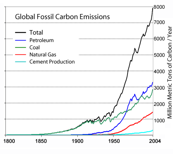
3. A source of historical fossil fuel usage. The further back this goes in time the better. I have two locations: one from the Wikipedia site on atmospheric CO2 (Image) or one from the NOAA site.
4. A probability density function (PDF) for the CO2 impulse response (see the previous post). If you don't have this PDF, use the first-order reaction rate exponential function, R(t)=exp(-kt).
5. A convolution function, which you can do on a spreadsheet with the right macro [1].

The convolution of carbon production Pc(t) with the impulse response R(t) generates C(t):

C(t) = k*[Integral of Pc(t-x)*R(x) from x=0 to x=t] + L

Multiplying the result by a conversion factor k; then adding this to the baseline L generates the filtered Mauna Loa curve as a concentration in CO2 parts per million.

I used R(t)=exp(-t/T), where T=42 years and L=1280 ppm baseline for the following curve fit (using data from Figure 3 for Pc(t)) .

Figure 2: Convolution ala the Shock Model of the yearly carbon emission with an impulse response function. An analytical result from a power-law (N=4) carbon emission model is shown as a comparison..

For Figure 2, I also applied a curve fit model of the carbon generated, which followed a Time⁴ acceleration, and which had the same cumulative as of the year 2004 [2]. You can see subtle differences between the two which indicates that the rate function does not completely smooth out all the yearly variations in carbon emission (see Figure 3). So the two convolution approaches show some consistency with each other, but the fit to the Mauna Loa data appears to have a significant level shift. I will address this in a moment.

Figure 3: Carbon emission data used for Figure 2. A power-law starting in the year 1800 generates a smoothed idealized version of the curve useful for generating a closed-form expression.

The precise form of the impulse response function, other than the average rate selected, does not change the result too much. I can make sense out of this since the strongly increasing carbon production wipes out the fat-tails tails of slower order reaction kinetics (see Figure 4). In terms of the math, a Time⁴ power effectively overshadows a weak 1/sqrt(Time) or 1/Time response function. However, you will see start to see this tail if and when we start slowing down the carbon production. This will give a persistence in CO2 above the baseline for centuries.

Figure 4: Widening the impulse response function by dispersing the rates to the maximum entropy amount, does not significantly change the curvature of the CO2 concentration. Dispersion will cause the curve to eventually diverge and more closely follow the integrated carbon curve but we do not see this yet on our time scale.

Once we feel comfortable doing the convolution, we can add in a piecewise extrapolated production curve and we can anticipate future CO2 levels. We need a fat-tail impulse response function to see the long CO2 persistence in this case (unless 42 years is long enough for your tastes).

The Loose End

If you look at Figure 1, you can obviously see an offset of the convolution result from the actual data. This may seem a little puzzling until you realize that the background (pre-industrial) level of CO2 can shift the entire curve up or down. I used the background level of 280 ppm purely out of popularity reasons. More people quote this number than any other number. However, we can always evaluate the possibility that a higher baseline value would fit the convolution model more closely. Let's give that a try.

The following figure (adapted from here) shows a different CO2 data set which includes the Mauna Loa data as well as earlier proxy ice core data. Based on the levels of CO2, I surmised that the NOAA scientist that generated this graph subtracted out the 280ppm value and plotted the resultant offset. I replotted the data convolution as the dotted gray line.

Figure 5: The CO2 data replotted with extra proxy ice core data, assuming a 280ppm baseline (pre-industrial) level. The carbon production curve is also plotted. You can clearly see that the convolution of the impulse response results in a curve that has a consistent shift of between 10 and 20 ppm below the actual data.

Note that my curve consistently shows a shift 14ppm below the actual data (note the log-scale). This indicates to me that the actual background CO2 level sits 14ppm above 280ppm or at approximately 294ppm. When I add this 14ppm to the curve and replot, it looks like:

Figure 6: The convolution model replotted from Figure 5 with a baseline of 294ppm CO2 instead of 280. Note the generally better agreement to the subtle changes in slope

Although the data does not go through a wide dynamic range, I see a rather parsimonious agreement with the two parameter convolution fit.

Just like in the oil shock model, the convolution of the stimulus with an impulse response function will tend to dampen and shift the input perturbations. If you look closely at Figure 6, you can see faint reproductions of the varying impulse, only shifted by about 25 years. I contend that this "delayed ghosting" comes about directly as a result of the 42-year time constant I selected for the reaction kinetics rate. This same effect occurs with the well-known shift between the discovery peak and production peak in peak oil modeling. Even though King Hubbert himself pointed out this effect years ago, no one else has explained the fundamental basis behind this effect, other than through the application of the shock model. That climate scientists most assuredly use this approach as well points out a potential unification between climate science and peak oil theory. I know David Rutledge of CalTech has looked at this connection closely, particularly in relation to future coal usage.

Bottom Line

To believe this model, you have to become convinced that 294 ppm is the real background pre-industrial level (not 280), and that 40 years is a pretty good time constant for CO2 decomposition kinetics. Everything else follows from first-order rate laws and the estimated carbon emission data.

Of course, this simple model does not take into possible positive feedback effects, yet it does give one a nice intuitive framework to think about how hydrocarbon production and combustion leads directly to atmospheric CO2 concentration changes and ultimately climate change. Doing this exercise has turned into an eye-opener for me, as it didn't really occur to me how straightforward one can derive the CO2 results. Gore had it absolutely right.


Update: From the feedback from some astute TOD readers, it has become clear that some other forcing inputs could easily make up the 14 ppm offset. Changing agriculture and forestry patterns, and other human modifications of the biota could alter the forcing function during the 200+ year time-span since the start of the industrial revolution. Although recyclable plant life should eventually become carbon neutral, the fat-tail of the CO2 impulse response function means that sudden changes will persist for long periods of time. A slight rise from time periods from before the 1800's coupled with an extra stimulus on the order of 500 million tons of carbon per year (think large-scale clearcutting and tilling from before and after this period) would easily close the 14 ppm CO2 gap and maintain the overall fit of the curve.

However, we would need to apply the fat-tail response function, g/(g+sqrt(t)), to maintain the offset for the entire period.

Another comment by EoS:

I don't think it is useful to think of an average CO2 lifetime. That implies a lumped linear model with only a single reservoir, hence an exponential decay towards equilibrium. In reality there are lots of different CO2 reservoirs with different capacities and time constants. So any lumped model had better use several reservoirs with widely varying time constants at a minimum, or else it will get the time behavoir seriously wrong.

It turns out that the variation or dispersion in reaction rates makes very little difference in the slope on the climb up. That is fundamental and I addressed that in Figure 4. The reason for this is very simple mathematics -- the climb up in CO2 is generated by power laws on the order of N>3 or by exponential increases. That is the nature of accelerating fossil fuel usage. In contrast the reaction rates of CO2 have exponents that are negative or have inverse power laws of very low order, the so-called fat-tail distributions. When you put these together, the power law increase essentially crushes the long-tails and all you see are the average value of the faster kinetics. I put in the analytical solution so you can see this directly in the convolution results.

Alternately, apply a simple convolution of accelerating growth [exp(at)] with a first-order reaction decline [exp(-kt)] and you will see what I mean. You get this:

C(t) = (exp(at)-exp(-kt)/(a+k)

The accelerating rate a will quickly overtake the decline term k. If you put in a spread in k values as a distributed model, the same result will occur. That essentially demonstrates Figure 4. Climate scientists should realize this as well since they have known about the uses of convolution in the carbon cycle for years (see chapter 16 in "The carbon cycle" by T. M. L. Wigley and David Steven Schimel).

Yet, if we were to stop burning hydrocarbons today, then we would see the results of the fat-tail decline. Again, I think the climate scientists understand this fact as well but that idea gets obscured by layers of computer simulations and the salient point or insight doesn't get through to the layman. This is understandable because these are not necessarily intuitive concepts.

This following figure models CO2 uptake if we suddenly stop growing fossil fuel use after the year 2007. We don't simple stop using oil and coal, we simply keep our usage constant.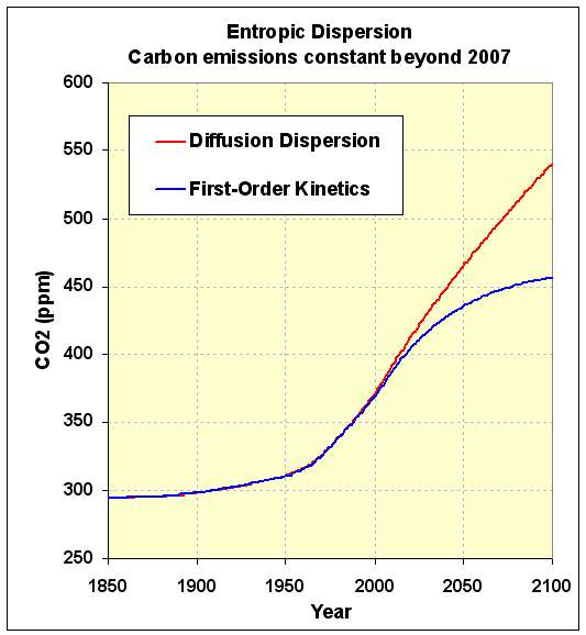

Figure 7: Extrapolation of slow kinetics vs fat-tail kinetics

Up to that point in time a dispersive (i.e. variable) set of rate kinetics will be virtually indistinguishable from a single rate (see Figure 4). And you can see that behavior as the curves match for the same average rate. But once the growth increase is cut off, the dispersive/diffusive kinetics takes over and the rise continues. With the first-order kinetics the growth continues but it becomes self-limiting as it reaches an equilibrium. (see http://mobjectivist.blogspot.com/2010/04/fat-tail-in-co2-persistence.html). This works as a plain vanilla rate theory with nothing by the way of feedbacks in the loop. When we include a real positive feedback, that curve can even increase more rapidly.

Recall that this analysis carries over from studying dispersion in oil discovery and depletion. The rates in oil depletion disperse all over the map, yet the strong push of technology acceleration essentially narrows the dispersed elements so that we can get a strong oil production peak or a plateau with a strong decline. In other words, if we did not have the accelerating components, we would have had a long drawn out usage of oil that would reflect the dispersion. That explains why I absolutely hate the classical derivation of the Hubbert Logistics curve, as it reinforces the opinion of peak oil as some "single-rate" model. In fact just like climate science, everything gets dispersed and follows multiple pathways, and we need to use the appropriate math to analyze that kind of situation.

Climate scientists understand convolution, but peak oil people don't, except when you apply the shock model.

That basically outlines why I want to share these ideas with climate scientists and unify the concepts. It will help both camps, simply by dissemination of fresh ideas and unification of the strong ones.

---

Notes:
[1] Excel VB convolution script

http://www.microsoft.com/communities/newsgroups/list/en-us/default.aspx?dg=microsoft.public.excel.worksheet.functions&tid=933752da-6f86-4af8-9dba-b9edf57f77d9&cat=en_us_b5bae73e-d79d-4720-8866-0da784ce979c&lang=en&cr=us&sloc=&p=1

Copy the function below into a regular codemodule, then use it like

=SumRevProduct(A2:E2,A3:E3)

It will work with columns as well as rows.

HTH,
Bernie
MS Excel MVP

Function SumRevProduct(R1 As Range, R2 As Range) As Variant
Dim i As Integer
If R1.Cells.Count <> R2.Cells.Count Then GoTo ErrHandler
If R1.Rows.Count > 1 And R1.Columns.Count > 1 Then GoTo ErrHandler
If R2.Rows.Count > 1 And R2.Columns.Count > 1 Then GoTo ErrHandler

For i = 1 To R1.Cells.Count
SumRevProduct = SumRevProduct + _
R1.Cells(IIf(R1.Rows.Count = 1, 1, i), _
IIf(R1.Rows.Count = 1, i, 1)) * _
R2.Cells(IIf(R2.Rows.Count = 1, 1, R2.Cells.Count + 1 - i), _
IIf(R2.Rows.Count = 1, R2.Cells.Count + 1 - i, 1))
Next i
Exit Function
ErrHandler:
SumRevProduct = "Input Error"
End Function

[2] Try this with Wolfram Alpha. It gets finicky sometimes but it does symbolic algebra fairly well.