Rayleigh Fading, Wireless Gadgets, and a Global Context

The intermittent nature of wind power that I recently posted on has a fundamental explanation based on entropy arguments. It turns out that this same entropy-based approach explains some other related noisy and intermittent phenomena that we deal with all the time. The obvious cases involve the use of mobile wireless gadgets such as WiFi devices, cell phones, and GPS navigation aids in an imperfect (i.e. intermittent) situation. The GPS behavior has the most interesting implications which I will get to in a moment.

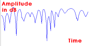
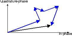
First of all, consider that we often use these wireless devices in cluttered environments where the supposedly constant transmitted power results in frustrating fade-outs that we have all learned to live with. An example of Rayleigh fading appears to the right. You can find some signal interference-based explanations for why this happens, originating via the same intentional phase cancellations that occur in noise-cancelling headphones. For the headphones, the electronics flip the phase so all interferences turn destructive, but for wireless devices, the interferences turn random, some positive and some negative, so the result gives the random signal shown.

In the limit of a highly interfering environment the amplitude distribution of the signal shows a Rayleigh distribution, the same observed for wind speed.

p(r) = 2kr exp(-kr²)

Because all we know about our signal is an average power, it occurred to me that one can use Maximum Entropy Principles to estimate the amplitude from the energy stored in the signal, just like one can derive it for wind speed. So, as a starting premise, if we know the average power alone, then we can derive the Rayleigh distribution.

The following figure (taken from here) shows the probability density function of the correlated power measured from a GPS signal. Since power in an electromagnetic signal relates to energy as a flow of constant energy per unit time, then we would expect the energy or power distribution to look like a damped exponential, in line with the maximum entropy interpretation. And sure enough, it does exactly match a damped exponential (note that the Std Dev = Mean, a dead giveaway for an exponential distribution).

p(E) = k*exp(-kE)

Yet since power (E) is proportional to Amplitude squared (r ²), we can derive the probability density function by invoking the chain rule.

p(A) = p(E)*dE/dr = exp(-kr²) * d(r²)/dr = 2kr * exp(-kr²)

which precisely matches the Rayleigh distribution, implying that Rayleigh fits the bill as a Maximum Entropy (MaxEnt) distribution. So too does the uniformly random phase in the destructive interference process qualify as a MaxEnt distribution, which will range from 0 to 360 degrees (which gives an alternative derivation of Rayleigh). So all three of these distributions, Exponential, Rayleigh, and Uniform all act together to give a rather parsimonious application of the maximum entropy principle.

The most interesting implication of an entropic signal strength environment relates to how we deal with this power variation in our electronic devices. If you own a GPS, you know this when when trying to acquire a GPS signal from a cold-start. The amount of time it takes to acquire GPS satellites can range from seconds to minutes, and sometimes we don't get a signal at all, especially if we have tree cover with branches swaying in the wind.

Explaining the variable delay in GPS comes out quite cleanly as a fat-tail statistic if you understand how the GPS locks into the set of satellite signals. The solution assumes the entropy variations of the signal strength and integrating this against the search space that the receiver needs to lock-in to the GPS satellites.

Since the search space involves time on one axis and frequency in the other, it takes in the limit ~N² steps to decode a solution that identifies a particular satellite signal sequence for your particular unknown starting position [1]. This gets reduced because of the mean number of steps needed on average in the search space. We can use some dynamic programming matrix methods and parallel processing (perhaps using an FFT) to get this to order N, so the speed-up for a given rate is t². So this will take a stochastic amount of time according to MaxEnt of :

P (t | R) = exp(-c*R*t²)

However because of the Rayleigh fading problem we don't know how long it will take to integrate our signal with regard to the rate R. This rate has a density function proportional to the power level distribution :

p (R) = k * exp(-k*R)

then according to Bayes the conditionals line up to give the probability of acquiring a signal within time t:

P (t) = integral of P(t |R) * p(R) over all R

this leads to the entropic dispersion result of:

P (t < T) = 1/(1+(T/a)²)

where a is an empirically determined number derived from k and c. I wouldn't consider this an extremely fat tail because the acceleration of the search by quadrature tends to mitigate very long times.

I grabbed some data from a GPS project that has a goal to speed up wild-fire response times by cleverly using remote transponders : The FireBug project. They published a good chunk of data for cold-start times as shown in the histogram below. Note that the data shows many times that approach 1000 seconds. The single parameter entropic dispersion fit (a=62 seconds) appears as the blue curve, and it fits the data quite well:



Interesting how we can sharpen the tail in a naturally entropic environment by applying an accelerating technology (also see oil discovery). Put this in the context of a diametrically opposite situation where the diffusion limitations of CO2 slow down the impulse response times in the atmosphere, creating huge fat-tails which will inevitably lead to global warming.

If we can think of some way to accelerate the CO2 removal, we can shorten the response time, just like we can speed up GPS acquisition times or speed up oil extraction. Or should we have just slowed down oil extraction to begin with?

How's that for some globally relevant context?

---

Notes:

[1] If you already know your position and have that stored in your GPS, the search time shrinks enormously. This is the warm or hot-start mode that is currently used by most manufacturers. The cold-start still happens if you transport a "cold" GPS to a completely different location and have to re-ascquire the position based on unknown starting coordinates.

The Fat-Tail in CO2 Persistence

I constantly read about different estimates for the "CO2 Half-Life" of the atmosphere. I have heard numbers as short as 6 years and others as long as 100 years or more.

ClimateProgress.org -- Strictly speaking, excess atmospheric CO2 does not have a half-life. The distribution has a very long tail, much longer than a decaying exponential.

As an approximation, use 300-400 years with about 25% ‘forever’.
....
ClimateProgress.org -- David is correct. Half-life is an inappropriate way to measure CO2 in the atmosphere. The IPCC uses the Bern Carbon Cycle Model. See Chapter 10 of the WG I report (Physical Basis) or http://www.climate.unibe.ch/ ~joos/ OUTGOING/ publications/ hooss01cd.pdf

This issue has importance because CO2 latency and the possible slow retention has grave implications for rebounding from a growing man-made contribution of CO2 to the atmosphere. A typical climate sceptic response will make the claim for a short CO2 lifetime :

Endangerment Finding Proposal
Lastly; numerous measurements of atmospheric CO2 resident lifetime, using many different methods, show that the atmospheric CO2 lifetime is near 5-6 years, not 100 year life as stated by Administrator (FN 18, P 18895), which would be required for anthropogenic CO2 to be accumulated in the earth's atmosphere under the IPCC and CCSP models. Hence, the Administrator is scientifically incorrect replying upon IPCC and CCSP -- the measured lifetimes of atmospheric CO2 prove that the rise in atmospheric CO2 cannot be the unambiguous result of human emissions.

Not knowing a lot about the specific chemistry involved but understanding that CO2 reaction kinetics has much to do with the availability of reactants, I can imagine the number might swing all over the map, particular as a function of altitude. CO2 at higher altitudes would have fewer reactants to interact with.

So what happens if we have a dispersed rate for the CO2 reaction?

Say the CO2 mean reaction rate is R=0.1/year (or a 10 year half-life). Since we only know this as a mean, the standard deviation is also 0.1. Placing this in practical mathematical terms, and according to the Maximum Entropy Principle, the probability density function for a dispersed rate r is:

p(r) = (1/R) * exp(-r/R)

One can't really argue about this assumption, as it works as a totally unbiased estimator, given that we only know the global mean reaction rate.

So what does the tail of reaction kinetics look like for this dispersed range of half-lifes?

Assuming the individual half-life kinetics act as exponential declines then the dispersed calculation derives as follows

P(t) = integral of p(r)*exp(-rt) over all r

This expression when integrated gives the following simple expression:

P(t) = 1/(1+Rt)

which definitely gives a fat-tail as the following figure shows (note the scale in 100's of years). I can also invoke a more general argument in terms of a mass-action law and drift of materials; this worked well for oil reservoir sizing. Either way, we get the same characteristic entroplet shape.

Figure 1: Drift (constant rate) Entropic Dispersion

For the plot above, at 500 years, for R=0.1, about 2% of the original CO2 remains. In comparison for a non-dispersed rate, the amount remaining would drop to exp(-50) or ~2*10^-20 % !

Now say that R holds at closer to a dispersed mean of 0.01, or a nominal 100 year half-life. Then, the amount left at 500 years sits at 1/(1+0.01*500) = 1/6 ~ 17%.

In comparison, the exponential would drop to exp(-500/100) = 0.0067 ~ 0.7%

Also, 0.7% of the rates will generate a half-life of 20 years or shorter. These particular rates quoted could conceivably result from those volumes of the atmosphere close to the ocean.

Now it gets interesting ...

Climatologists refer to the impulse response of the atmosphere to a sudden injection of carbon as a key indicator of climate stability. Having this kind of response data allows one to infer the steady state distribution. The IPCC used this information in their 2007 report.

Current Greenhouse Gas Concentrations
The atmospheric lifetime is used to characterize the decay of an instanenous pulse input to the atmosphere, and can be likened to the time it takes that pulse input to decay to 0.368 (l/e) of its original value. The analogy would be strictly correct if every gas decayed according to a simple expotential curve, which is seldom the case.
...
For CO2 the specification of an atmospheric lifetime is complicated by the numerous removal processes involved, which necessitate complex modeling of the decay curve. Because the decay curve depends on the model used and the assumptions incorporated therein, it is difficult to specify an exact atmospheric lifetime for CO2. Accepted values range around 100 years. Amounts of an instantaneous injection of CO2 remaining after 20, 100, and 500 years, used in the calculation of the GWPs in IPCC (2007), may be calculated from the formula given in footnote a on page 213 of that document. The above-described processes are all accounted for in the derivation of the atmospheric lifetimes in the above table, taken from IPCC (2007).

Click on the following captured screenshot for the explanation of the footnote.

The following graph shows impulse responses from several sets of parameters using the referenced Bern IPCC model (found in Parameters for tuning a simple carbon cycle model). What I find bizarre about this result is that it shows an asymptotic trend to a constant baseline, and the model parameters reflect this. For a system at equilibrium, the impulse response decay should go to zero. I believe that it physically does, but that this model completely misses the fact that it eventually should decay completely. In any case, the tail shows huge amount of "fatness", easily stretching beyond 100 years, and something else must explain this fact.

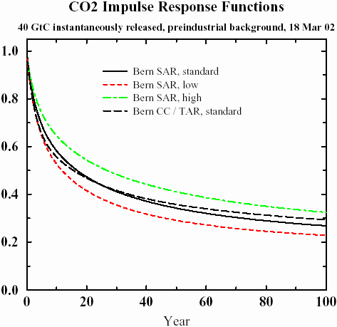
Figure 2: IPCC Model for Impulse Response

If you think of what happens in the atmosphere, the migration of CO2 from low-reaction rate regions to high-reaction rate regions can only occur via the process of diffusion. We can write a simple relationship for Fick's Law diffusion as follows:

dG(t)/dt = D (C(0)-C(x))/G(t)

This states that the growth rate dG(t)/dt remains proportional to the gradient in concentration it faces. As a volume gets swept clean of reactants, G(t) gets larger and it takes progressively longer for the material to "diffuse" to the side where it can react. This basically describes oxide growth as well.

The outcome of Fick's Law generates a growth law that goes as the square root of time - t ^1/2. According to the dispersion formulation for cumulative growth, we simply have to replace the previous linear drift growth rate shown in Figure 1 with the diffusion-limited growth rate.

P(t) = 1/(1+R*t ^1/2)

or in an alternate form where we replace the probability P(t) with a normalized response function R(t):

R(t) = a/(a+t ^1/2)

At small time scales, diffusion can show an infinite growth slope, so using a finite width unit pulse instead of a delta impulse will create a reasonable picture of the dispersion/diffusion dynamics.

Remarkably, this simple model reproduces the IPCC-SAR model almost exactly, with the appropriate choice of a and a unit pulse input of 2 years. The IPCC-TAR fit uses a delta impulse function. The analytically calculated points lie right on top of the lines of Figure 2, which actually makes it hard to see the excellent agreement. The window of low to high reaction rates generates a range of a from 1.75 to 3.4, or approximately a 50% variation about the nominal. I find it very useful that the model essentially boils down to a single parameter of entropic rate origin (while both diffusion and dispersion generates the shape) .

Figure 3: Entropic Dispersion with diffusional growth kinetics describes the CO2 impulse response function with a single parameter a. The square of this number describes a characteristic time for the CO2 concentration lifetime.

You don't see it on this scale, but the tail will eventually reach zero, but at a rate asympotically proportional to the square root of time. In 10,000 years, it will reach approximately the 2% level (i.e. 2/sqrt(10000)).

Two other interesting observations grow out of this most parsimonious agreement.

First of all, why did the original IPCC modelers from Bern not use an expression as simple as the entropic dispersion formulation? Instead of using a three-line derivation with a resultant single parameter to model with, they chose an empirical set of 5 exponential functions with a total of 10 parameters and then a baseline offset. That makes no sense unless their model essentially grows out of some heuristic fit to measurements from a real-life carbon impulse (perhaps data from paleoclimatology investigation of an ancient volcanic eruption; I haven't tracked this down yet). I can only infer that they never made the connection to the real statistical physics.

Secondly, the simple model really helps explain the huge discrepancy between the quoted short lifetimes by climate sceptics and the long lifetimes stated by the climate scientists. These differ by more than a magnitude. Yet, just by looking at the impulse response in Figure 3, you can see the fast decline that takes place in less than a decade and distinguish this from the longer decline that occurs over the course of a century. This results as a consequence of the entropy within the atmosphere, leading to a large dispersion in reaction rates, and the rates limited by diffusion kinetics as the CO2 migrates to conducive volumes. The fast slope evolving gradually into a slow slope has all the characteristics of the "law of diminishing returns" characteristic of diffusion, with the precise fit occurring because I included dispersion correctly and according to maximum entropy principles. (Note that I just finished a post on cloud ice crystal formation kinetics which show this same parsimonious agreement).

Think of it this way: if this simple model didn't work, one would have to reason why it failed. I contend that entropy and disorder in physically processes plays such a large role that it ends up controlling a host of observations. Unfortunately, most scientists don't think in these terms; they still routinely rely on deterministic arguments alone. Which gets them in the habit of using heuristics instead of the logically appropriate stochastic solution.

Which leads me to realize that the first two observations have the unfortunate effect of complicating the climate change discussion. I don't really know, but might not climate change deniers twist facts that have just a kernel of truth? Yes, "some" of the CO2 concentrations may have a half-life of 10 years, but that misses the point completely that variations can and do occur. I am almost certain that sceptics that hang around at sites like ClimateAudit.org see that initial steep slope on the impulse response and convince themselves that a 10 year half-life must happen, and then decide to use that to challenge climate change science. Heuristics give the skilled debater ammo to argue their point any way they want.

I can imagine that just having the ability to argue in the context of a simple entropic disorder can only help the discussion along, and relying on a few logically sound first-principles models provides great counter-ammo against the sceptics.

One more thing ...

So we see how a huge fat tail can occur in the CO2 impulse response. What kind of implication does this have for the long term?

Disconcerting, and that brings us to the point that the point that climate scientists have made all along. With a fat-tail, one can demonstrate that a CO2 latency fat-tail will cause the responses to forcing functions to continue to get worse over time.

As this paper notes and I have modeled, applying a stimulus generates a non-linear impulse response which will look close to Figure 3. Not surprisingly but still quite disturbing, applying multiple forcing functions as a function of time will not allow the tails to damp out quickly enough, and the tails will gradually accumulate to a larger and larger fraction of the total. Mathematically you can work this out as a convolution and use some neat techniques in terms of Laplace or Fourier transforms to prove this analytically or numerically.

This essentially explains the 25% forever in the ClimateProgress comment. Dispersion of rates essentially prohibit the concentrations to reach a comfortable equilibrium. The man-made forcing functions keep coming and we have no outlet to let it dissipate quickly enough.

I realize that we also need to consider the CO2 saturation level in the atmosphere. We may asymptotically reach this level and therefore stifle the forcing function build-up, but I imagine that no one really knows how this could play out.

As to one remaining question, do we believe that this dispersion actually exists? Applying Bayes Theorem to the uncertainty in the numbers that people have given, I would think it likely. Uncertainty in people's opinions usually results in uncertainty (i.e. dispersion) in reality.

This paper addresses many of the uncertainties underlying climate change: The shape of things to come: why is climate change so predictable?

The framework of feedback analysis is used to explore the controls on the shape of the probability distribution of global mean surface temperature response to climate forcing. It is shown that ocean heat uptake, which delays and damps the temperature rise, can be represented as a transient negative feedback. This transient negative feedback causes the transient climate change to have a narrower probability distribution than that of the equilibrium climate response (the climate sensitivity). In this sense, climate change is much more predictable than climate sensitivity. The width of the distribution grows gradually over time, a consequence of which is that the larger the climate change being contemplated, the greater the uncertainty is about when that change will be realized. Another consequence of this slow growth is that further eff orts to constrain climate sensitivity will be of very limited value for climate projections on societally-relevant time scales. Finally, it is demonstrated that the e ffect on climate predictability of reducing uncertainty in the atmospheric feedbacks is greater than the eff ect of reducing uncertainty in ocean feedbacks by the same proportion. However, at least at the global scale, the total impact of uncertainty in climate feedbacks is dwarfed by the impact of uncertainty in climate forcing, which in turn is contingent on choices made about future anthropogenic emissions.

In some sense, the fat-tails may work to increase our certainty in the eventual effects -- we only have uncertainty in the when it will occur. People always think that fat-tails only expose the rare events. In this case, they can reveal the inevitable.

---

Added Info:

Segalstad pulled together all the experimentally estimated residence times for CO2 that he could find, and I reproduced them below. By collecting the statistics for the equivalent rates, it turns out that the standard deviation approximately equals the mean (0.17/year) -- this supports the idea that the uncertainty in rates found by measurement matches the uncertainty found in nature, thus giving the entropic fat tail. These still don't appear to consider diffusion, which fattens the tail even more.

Authors [publication year]	Residence time (years)
Based on natural carbon-14
Craig [1957]	7 +/- 3
Revelle & Suess [1957]	7
Arnold & Anderson [1957]including living and dead biosphere	10
(Siegenthaler,1989)	4-9
Craig [1958]	7 +/- 5
Bolin & Eriksson [1959]	5
Broecker [1963], recalc. by Broecker & Peng [1974]	8
Craig [1963]	5-15
Keeling [1973b]	7
Broecker [1974]	9.2
Oeschger et al. [1975]	6-9
Keeling [1979]	7.53
Peng et al. [1979]	7.6 (5.5-9.4)
Siegenthaler et al. [1980]	7.5
Lal & Suess [1983]	3-25
Siegenthaler [1983]	7.9-10.6
Kratz et al. [1983]	6.7
Based on Suess Effect
Ferguson [1958]	2 (1-8)
Bacastow & Keeling [1973]	6.3-7.0
Based on bomb carbon-14
Bien & Suess [1967]	>10
Münnich & Roether [1967]	5.4
Nydal [1968]	5-10
Young & Fairhall [1968]	4-6
Rafter & O'Brian [1970]	12
Machta (1972)	2
Broecker et al. [1980a]	6.2-8.8
Stuiver [1980]	6.8
Quay & Stuiver [1980]	7.5
Delibrias [1980]	6
Druffel & Suess [1983]	12.5
Siegenthaler [1983]	6.99-7.54
Based on radon-222
Broecker & Peng [1974]	8
Peng et al. [1979]	7.8-13.2
Peng et al. [1983]	8.4
Based on solubility data
Murray< (1992)	5.4
Based on carbon-13/carbon-12 mass balance
Segalstad (1992)	5.4

Dispersive and non-dispersive growth in ice crystals

I have wanted to do a post on the growth of crystals for a while. Although on a totally different size scale (microns) and time scale (hours) than that of oil reservoir growth (million barrels and eons/ages), the essential behavioral notions behind the two cases of growth remain much the same.

I suggest that in the most disordered environments, the role of entropy overrides other factors enough so that some simple dispersion arguments can explain the size distribution completely.

Take as an example the formation of ice crystals in a cirrus cloud. Depending on the surrounding temperature a crystal nucleates on some foreign particle and then starts growing. The atmospheric conditions have enough variety that the growth rate will disperse to the maximum entropy amount given a mean rate value. The end state for volumetric growth will also show the same amount of variation. Put these two factors together and we end up with the same size distribution as we have for oil reservoir sizes.

p(x) = S/(S + x)²

where x is the size variate and S is the mean size. This becomes the entroplet form of a probability density function. Plotting this on a logarithmic size scale, the envelope looks the following. I roughly plotted how the dispersed velocity components play into the aggregation of the full profile (note that this serves as a mirror image of the other way of thinking about growth, that of varying end-states).

In some sense, the entroplet aggregates the non-dispersed rate functions which show individually much steeper exponential declines. Graphically, these individual curves do not stand-out on their own since the entropic disorder smooths and disperses the curves efficiently. Keep this in mind for a moment.

The following particle size distribution (PSD) graph shows measurements taken from high altitude cloud experiments. The size gets measured along a single length dimension and the density of the particles takes the place of a probability. I assume that they have plotted the density as a mass function along the x-axis. I convert this to a volumetric size growth problem, integrate the growth for a time duration corresponding to the cloud formation period, and plot the entropic dispersion model result below. The value for S is 2 and the integration scale is 16 (see Note [1]) .

Particle Size Distributions
Cloud ice particle number density n(D) vs. the long dimension of particles as observed at the temperature range of -25° C and -30° C [from Platt, 1997]. It shows a bimodal structure in the ice crystal distribution with the second peak at ~500 mm (edit: microns).

The data fits the entropic dispersion model nicely (green line), but notice at low density that an extra mode shows up as the blue line. This clearly has a sharp exponential drop so likely has a non-dispersive origin. In terms of the higher density entropic model, this stands out as an ordered nucleation regime in the midst of a sea of disordered ice crystal growth modes. Compare to the first figure again and one can see how a distinct peak could occur.

Why or how physically can this bump occur? One can understand this in the context of a completely unrelated analysis, that of marathon finishing times. In a race composed of ordinary citizens, mixed in with some elite runners (bribed by prize money), the elites will form a low density bump in a histogram of finishing times.

The incentives and training and good genetics of the elites separate them from the recreational athlete enough so that they generate a statistically measurable deviation from the trend. Anyone who follows sports understands how this can happen.

I assert that an ice crystal growth model could show this same behavior. Some unknown nucleation process has provided an optimal growth environment for these crystals to deviate from the entropic distribution. Hypothesizing, this could take the form of a catalyst or an accommodating growth substrate. With a power tail of -3/2 this might well have a strong diffusive growth component. However, the nuclei occur rarely enough so they do not drown out the much more common random or spontaneously occurring growth centers. It thus shows up as a clear non-dispersive growth mode in a sea of non-uniformity.

On a micro-level, we do have a variety of reproducible structured shapes to bind against. I would predict that nothing like this would ever happen on the scale of oil reservoirs, black swans notwithstanding. On the scale of oil reservoirs, no two substrates will ever have a common origin, so that the entropic trends will dominate.

BTW, I hope this original analysis may prove of some help to those looking at cloud-based climate change forcing functions, or particle size distributions of volcanic ash (see right). It opens up some possibilities to thinking in a different way. From the plot on the Wikipedia page, they use a log-normal fit to the data yet one that uses an entropic dispersion formulation with the appropriate volume/diameter exponent often can work just as well. Below, I use a root 1/2 on volume on dispersive growth which may indicate a diffusion-controlled rate.

---

Notes

[1] The approach described here, which essentially broadens the peak but retains the power law tail. Convert the linear growth to a time varying parameter (x=kt) and then treat the growth as an evolving pattern which starts from multiple points in time as the cloud develops.

P(x) = Average 1/(1+S/(k*t)) from t=T to t=T+x/k

This is a cumulative so take the derivative with respect to x to get the PDF.

p(x) ~ 1/(S+x) - 1/(S+kT+x)

As described in the reference, this broadening also applies to species diversification and for oil field growth. The only complicating factor in this analysis is that oil reservoir is a volume, yet crystal sizes get reported as a length and we have to convert that to a volume. This means the derivative has to include a chain rule to convert the volume x to a length parameter L, x ~ L³ generates dx/dL ~ L².

Extracting the Learning Curve in Labor Productivity Statistics

The term ergodicity refers to the uniformity and fairness in occupation of a system of probability-based states. In the way I think about it, an ergodic Tic-Tac-Toe distribution would have gained enough statistics such that the average measured occupancy of squares of an averaged game's end would equal the probability of some theoretically predicted occupancy.

One can get to this state either by capturing statistics over a long period of time or having some process that doesn't have statistical runs that break the stationarity principle. I sometimes confuse the term stationary with ergodic. The first has more to do with suggesting that a particular snapshot in time does not differ from another snapshot at some later time (i.e. independent events). The latter makes certain that the process has enough variety in its trajectories to visit all the possible states.

One of the first mathematical experiments I remember working in school had to do with random number generation. At the time, hand-held calculators still held some excitement and to take advantage of this, the instructor gave the students an assignment to come up with their own uniform random number generator by creating some complicated algorithm on the calculator. The student could then easily test his results.

As I recall, I felt a certain amount of pride in the clever way that I could get results that appeared random. I don't think I understood what pseudo-random meant at the time. In retrospect, I probably had enough knowledge to realize the power of the inverse trig functions and how they could generate numbers between zero and one, and of the idea of truncating to the decimal part of the number (to get a value between 0 and 1). I am sure that my classroom random number generator would not pass any quality tests, but it worked well enough for learning purposes.

I mention this because I also think it first gave me an idea of how easy one can enter into a very disordered state, and one of almost "uniform randomness". It really does not take much in terms of a combination of linear or non-linear calculations before one can obtain a well-travelled set of trajectories and thus an ergodic distribution that also seems to meet the maximum entropy principle.

The post on Japanese labor productivity statistics rests on this same assumption. Enough variety exists in the set of Japanese labor pool for the statistics to reach an ergodic level. And enough complexity exists in the ways that the laborers operate that they will visit all the labor productivity states possible considering the constraints. That partly explains why I can get confidence that some deep fundamental stochastic behavior explains the results.

The labor productivity model that I used to generate the distribution involved the application of a non-linear Lanchester model for competition. The non-linear nature of this model at least contributes to the potential for the states to reach an ergodic limit. Much like a complex expression invoked on a calculator allows one to generate quite easily a pseudo-random distribution.

In the parlance of attractors, these equations naturally translate into a scenario where you can imagine all sorts of possible trajectories to occur:
Unfortunately, this does not help too much with intuition. Yes one can execute a bunch of random calculations and note how easily various states accumulate, but the non-linear math still gets in the way.

For that reason, I will create an alternate model of labor productivity that invokes similar math but relies on the more intuitive concept of a "learning curve". In practice, a learning curve can exist where a worker can pick up much of the rudimentary skills very quickly, yet to get that last level of productivity will often take much more time [1].

Call the labor productivity C(t) and note that it has some minimum (Max) and maximum level (Min) based on the basic minimum requirements of the company and on the maximum technically achievable productivity.

Then over the course of time, a new hire may see productivity rise according to this simple relationship:

dC(t) = k/(C(t) + v) * dt

This mathematical relationship says that the increment of productivity (dC) per unit of time (dt) is inversely proportional to the productivity accumulated so far. In this case productivity equates to skill level. Thus, the worker can learn the early skills very easily, where the accumulated skills have not risen to a high level. (The parameter v prevents the learning curve rate from going to infinity initially). However, as time advances and these skills accumulate, the growth of new skills starts to slow and it reaches something of an asymptotic limit. We can consider this a law of diminishing returns as the weight of the accumulated skills starts to weigh down the worker.

Rearranging the equation, we get:

(C + v) dC = k dt

We can integrate this to get the result:

½C² + vC= t + constant

This results in the same constraint relationship that I used in the previous post in determining P(C) according to the dispersion formulation for C. The equation if given constrained limits (both Max and Min values) has a solution according to the basic quadratic formula which I used for the Monte Carlo simulation. Otherwise we simply use the ergodic view that all the various values of t will get visited over time, and all the possible constant values will show up according to maximum entropy.

The following figure shows a single instance of a labor productivity learning curve. This has a minimum level and a maximum level at which productivity clamps to. Imagine a set of many of these curves, all with different quadratic slope and maximum constraint and that turns into the statistical mechanics of the labor productivity distribution function for P(C) that we see aggregated over all possible learning times.



which leads to this density function and the excellent fit to the data when entropic dispersion gets applied.


This essentially gives an alternate explanation as a learning curve problem for the excellent fit we get for labor productivity. All workers go through a learning curve that shows a minimum proficiency and a maximum productivity that clamps the level, in between we see the quadratic solution growth which shows up as the inverse power law of 2 in the labor productivity distribution function.

To have it make sense with the Lanchester model labor model, the warfare between firms competing for the same resources provide further elements of disorder. Workers switching firms can cause labor productivity to clamp as progress stalls. By the same token, the cross-pollination of worker skills between firms and of compounding growth adds to the dispersion in the growth rates.

---

[1] Also see Fick's diffusion equation or a random walk, which shows the same quasi-asympotic properties.

Telegraphing Monkeys, Entropy, and 1/f Noise

Onward with my entropy-based theory of everything.

The observed behavior known as 1/f noise seems to show up everywhere. They call it 1/f noise (also known as flicker or pink noise) because it follows an inverse power law in its frequency spectrum. It shows up both in microelectronic devices as well as emanating from deep space. Its ubiquity gives it an air of mystery and the physicist Bak tried to explain it in terms of self-organized critical phenomena. No need for that level of contrivance, as ordinary entropic disorder will work just as well.

That as an introduction, I have a pretty simple explanation for the frequency spectrum based on a couple of maximum entropy ideas.

The first relates to the origin of the power law in the frequency spectrum.

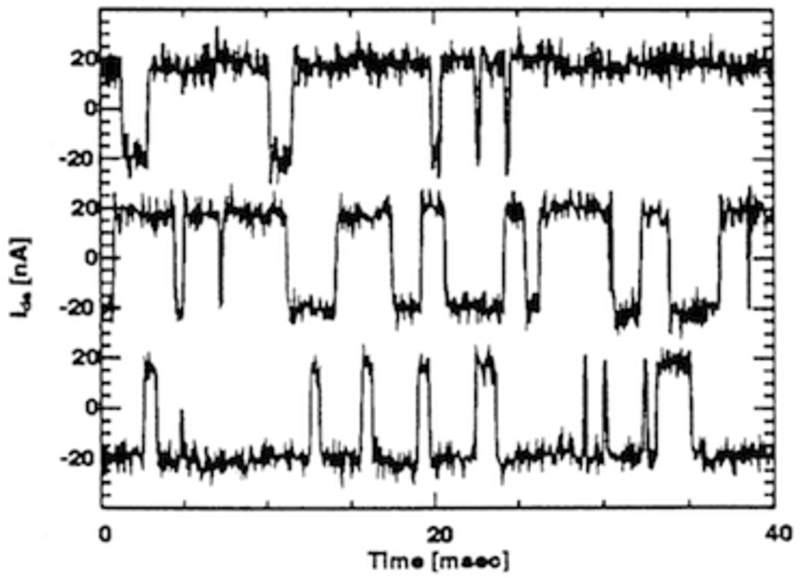
Something called random telegraph noise (RTS) (or burst or popcorn noise) can occur for a memory-less process. One can describe RTS by simply invoking a square-wave that has a probability of B to switch states at any dt time interval. This turns into a temporal Markov Chain kind of behavior and the typical noise measurement looks like the following monkeys-typing-at-a-telegraph trace and sounds like popcorn popping in its randomness. It pretty much describes an ordinary Poisson process.

The Markov Chain pulse train as described as above has an autocorrelation function that looks like a two-sided damped exponential. The correlation time equals 1/B.
The autocorrelation (or self convolution) of a stochastic statistical has some interesting properties. In this case, it does have maximum entropy content for the two-sided mean of 1/B -- MaxEnt for the positive axis and MaxEnt for the negative axis.

In addition, the Fourier Transform of the autocorrelation gives precisely the frequency power spectrum. This comes out proportionately to:

S(w) = sqrt(2/π) / (B²+w²)

where w is the angular frequency. The figure below shows the B=1 normalized Mathematica Alpha result.

That result only gives one spectrum of the many Markov switching rates that may exist in nature. If we propose that B itself can vary widely, we can solve for the superstatistical RTS spectrum.

Suppose that B ranged from close to zero to some large value R. We don't have a mean but we have these two limits as constraints. Therefore we let maximum entropy generate a uniform distribution for B.

To get the final spectrum, we essentially average the RTS spectrums over all possible intrinsic rates:

Integrate S(w|B) with respect to B from B=0 to B=R.

This generates the following result

S ' (w) = arctan(R/w)/w

If R becomes large enough then the arctan converges to a constant π/2 and reduces to the 1/f spectrum if we convert w=2π*f.

S ' (f) ~ 1/f

If we reduce R in the limit, then we get a regime that has a 1/f component and a 1/f ² above the R transition point, where it reverts back to a telegraph noise power-law.


An excellent paper by Edoardo Milotti, titled 1/f noise: a pedagogical review does a very good job of eliminating the mystery behind 1/f noise. He takes a slightly different tact but comes up with the same result that I have above.

In this review we have studied several mechanisms that produce fluctuations with a 1/f spectral density: do we have by now an "explanation" of the apparent universality of flicker noises? Do we understand 1/f noise? My impression is that there is no real mistery behind 1/f noise, that there is no real universality and that in most cases the observed 1/f noises have been explained by beautiful and mostly ad hoc models.

Milotti essentially disproved Bak's theory and said that no universality stands behind the power-law, just some common sense.

From Wikipedia

There are no simple mathematical models to create pink noise. It is usually generated by filtering white noise.

There are many theories of the origin of 1/ƒ noise. Some theories attempt to be universal, while others are applicable to only a certain type of material, such as semiconductors. Universal theories of 1/ƒ noise are still a matter of current research.

A pioneering researcher in this field was Aldert van der Ziel.

I actually took a class from the professor years ago and handed in this derivation as a class assignment (we had to write on some noise topic). I thought I could get his interest up and perhaps get the paper published, but, alas, he muttered a negative with his Dutch accent.

Years later, I finally get my derivation out on a blog.

As Columbo would say, just one more thing.
If the noise represents electromagnetic radiation, then one can perhaps generate an even simpler derivation. The energy of a photon is E(f)=h*f where h=Plank's constant and f is frequency. According to maximum entropy, if energy radiation remains uniform through the frequency spectrum, then we can only get this result if we apply a 1/f probability density function:

E(f) * p(E(f)) = h*f * (1/f) = constant

Wind Dispersion and the Renewable Hubbert Curve

Most critics of wind energy points to the unpredictability of sustained wind speeds as a potential liability in widespread use of wind turbines. Everyone can intuitively understand the logic behind this statement as they have personally experienced the variability in day-to-day wind statistics.

However comfortably we coexist with the concept of "windiness", people don't seem to understand the mathematical simplicity behind the wind speed variability. Actually the complexity of the earth's climate and environment contributes to this simplicity (see my TOD posts Information and Crude Complexity and Dispersion, Diversity, and Resilience). I suggest that it also could prove useful to understand the dispersion of airborne particulates, such as what occurred in the aftermath of the Icelandic volcano.

Let me go through the derivation of wind dispersion in a few easy steps. I start with the premise that every location on Earth has a mean or average wind speed. This speed has a prevailing direction but assume that it can blow in any direction.

Next we safely assume that the kinetic energy contained in the aggregate speed goes as the square of its velocity.

E ~ v ²

This comes about from the Newtonian kinetic energy law ½mv² and it shows up empirically as the aeronautical drag law (i.e. wind resistance) which also goes as the square of the speed. (Note that we can consider E as an energy or modified slightly as a power, since the energy is sustained over time)

As usual, I apply the Principle of Maximum Entropy to the possible states of energy that exist and come up with a probability density function (PDF) that has no constraints other than a mean value (with negative speeds forbidden).

p(E) = k* exp(-kE)

where k is a constant and 1/k defines the mean energy. This describes a declining probability profile, with low energies much more probable than high energies. To convert to a wind dispersion PDF we substitute velocity for energy and simplify:

p(v)dv = p(E)dE

p(v) = p(E) * dE/dv = 2cv * exp(-cv ²)

This gives the empirically observed wind speed distribution, showing a peak away from zero wind speeds and a rapid decline of frequency at higher velocity. I would consider this as another variation of an entropic velocity distribution. Many scientists refer to it as a Rayleigh or Weibull distribution. The excellent agreement in the figure below between the model and empirical data occurs frequently.

Wiki Wind Power
The Weibull model closely mirrors the actual distribution of hourly wind speeds at many locations. The Weibull factor is often close to 2 and therefore a Rayleigh distribution can be used as a less accurate, but simpler model.
Distribution of wind speed (red) and energy (blue) for all of 2002 at the Lee Ranch facility in Colorado. The histogram shows measured data, while the curve is the Rayleigh model distribution for the same average wind speed.

The Wiki explanation pulls its punches by using the heuristic family of Weibull curves. The Rayleigh comes out as the simpler model because it derives from first principles and any deviation from the quadratic exponent seems a bit silly. In the following curve, 1.95 is for all practical purposes the same as 2.


Contrary to other distributions, the wind PDF does not qualify as a fat-tail distribution. This becomes obvious if you consider that the power-law only comes about from the reciprocal measure of time, and since we measure speed directly, we invoke the entropic velocity profile directly as well.

So the interesting measure relates to the indirect way that we perceive the variations in wind speed. Only over the span of time do we detect the unpredictability and disorder in speed -- whether by gustiness or long periods of calm.

We can then pose all sorts of questions based on the entropic wind speed law. For example, how long would we have to wait to generate an accumulated amount of energy?

We can answer this analytically by simply equating the steady-state wind speed to a power and then integrating over all possibilities of the distribution that meet the minimum accumulated energy condition over a period of time.

The naive answer is trivial with the time PDF turning into the following fat-tail power-law:

p(t | E>cv ²) = (cv ²) * exp(-cv ²/ t ) / t ²

This equation corresponds to the following graphed probability density function (where we set an arbitrary E of cv ² = 25). It basically illustrates the likelihood of accumulating a specific energy goal within a given Time.


Because of the scarcity of high wind speeds and the finite time it takes to accumulate energy, one observes a short ramp-up to the peak. Typical wind-speeds round out the peak and the relatively common slow speeds contribute to the long fat-tail.

But since power has an extra velocity factor (Power = Drag*velocity, see Betz' law), it takes longer to integrate the low power values and the exponent changes from a quadratic value of 2 to a value of 5/3, via a chain rule.

p(t ) = (2*d/3) * exp(-d / t ^2/3 ) / t ^5/3

Thanks to E.Swanson at TOD for pointing this out. As you can see in the graph below, the fat-tail becomes fatter and the ramp-up a bit sooner for roughly the same peak value.
That gives us the power-law and a shape that looks surprisingly close to the time depletion curve for an oil reservoir. In fact, since probabilities have such universal properties, the curvature of this profile has the same fundamental basis as the Hubbert oil depletion profile. The huge distinction lies in the fact that wind energy provides a renewable source of energy, whereas oil depletion results in a dead-end.

So the hopelessness of the Hubbert curve when applied to Peak Oil turns to a sense of optimism when you realize that wind power generates a case of a Renewable Hubbert Curve. In other words, anytime you spin-up the wind-turbine you can always obtain a mini Hubbert cycle, if you have patience, just like you need patience with a train schedule.

Amazing the power of a simple consistent model; both dispersive discovery and the entropic wind dispersion model use the same set of ideas from probability. I find it unfortunate that not enough analysts can see through the complexity and discover the underlying elegance and intuitive power of simple entropy arguments.

---

Found recently:

http://www.theoildrum.com/node/6386#comment-613465
Once upon a time, long ago and not all that far away, I got an F in math at a famous engineering school because I simply wrote down the answer to a problem on the final instead of going thru all the tedious procedures. I complained to the TA that the answer was obvious and I didn't need the procedure. He said "Ya didn't show that you had learned the procedure, and so the F stays".

I then went down that long soulless hallway to the office of the SUMG (short ugly math genius) who took one glance at the problem and sneered "don't bother me with such trivia, the answer is obviously--". So I went back to the TA with this, and he answered "no procedure, no grade."

So---I look at wind turbines and think "sure this thing works, and it has a energy return of maybe 20 to 40 as is, and there are obvious ways to make it better. That's good enough, so let's go for it".

Right on.

Power Laws and Entrophic Systems

Every time I look at a distribution of some new set of data I come across, I can't help but notice a power law describing the trend. Also known as fat-tail distributions, NN Taleb popularized these curves with his book The Black Swan. Curiously, both he and Benoit Mandelbrot, his mentor, never spent much time pursuing the rather simple explanation for the classic 1/X cumulative distribution, often known as Zipf's Law or the Mandelbrot/Zipf variant.

That drives me crazy, as I don't consider making the assertion of the fat-tail's origin a huge academic risk. To me, I find that a power law invariably comes about when you invert a measure that follows a Poisson or exponential distribution with respect to its dimension. For example, a velocity distribution that shows a damped exponential profile, when inverted to the time dimension will give a fat-tail power law. I call that entropic velocity dispersion. See the last post on train scheduling delays to appreciate this.

So why doesn't anyone understand this rather simple transform and the general concept of power laws? Let us go through the various disciplines.

The Statistician: Hopes that everything will fall into a normal Gaussian distribution, so they can do their classical frequentist statistical analysis. Many show wariness of Bayesian analysis, of which the Maximum Entropy Principle falls into. This pollutes their pure statistics with the possibility of belief systems or even physics. Likes to think in terms of random walk, which almost always puts them in the time-domain and they can then derive their Poisson or Gaussian profiles with little effort. They need to usually explain fat-tails by Levy walks, which curiously assumes a power law as a first premise. So they never get the obviousness of the natural power law.

The Physicist: Wants to discover new laws of nature and thus directs research to meet this goal. Over the years, physicists have acquired the idea that power-laws somehow connect to critical phenomena, and this has gotten pounded into their skulls. Observing critical phenomena usually holds out hope that some new state of matter or behavior would reveal itself. So associating a power law within a controlled experiment of some phase transition offers up a possible Nobel Prize. They thus become experts at formulating an expression and simplifying it so that a power-law trend shows up in the tail. They want to discover the wondrous when the mundane explanation will just as easily do.

The Mathematician: Doesn't like probability too much because it messes up their idealized universe. If anything, they need problems that can challenge their mind without needing to interface to the real world. Something like Random Matrix Theory, which may explain velocity dispersion but within an N-dimensional state space. Let the Applied Mathematician do the practical stuff.

The Applied Mathematician: Unfortunately, no one ever reads what Applied Mathematicians have to say because they write in journals called Applied Mathematics, where you will find an article on digital image reconstruction calculation next to a calculation of non-linear beam dynamics. How would anyone searching for a particular solution find this stuff in the first place? (outside of a Google search that is)

The Engineer: Treats everything as noise and turbulence which gets in their way. They see 1/f noise and only want to get rid of it. Why explain something if you can't harness its potential? Anyways, if they want to explain something they can just as easily use a heuristic. Its just fuzzy logic at its core. For the computational engineer, anything else that doesn't derive from Fokker-Planck, Poisson's Equation, or Navier-Stokes is suspect. For the ordinary engineer, if it doesn't show up in the Matlab Toolbox it probably doesn't exist.

The Economist and The Quantitative Analyst: Will invoke things like negative probabilities before they use anything remotely practical. Math only serves to promote their economic theory predicting trends or stability, with guidance from the ideas of econometrics. Besides, applying a new approach will force them to sink the costs of years of using normal statistics. And they should know the expense of this because they invented the theory of sunk costs. The economist is willing to allow the econophysicist free reign to explore all the interesting aspects of their field.

I wrote this list at least partly tongue-in-cheek because I get frustrated by the amount of dead-end trails that I see scientists engaged in. They get tantalizingly close with ideas such as superstatistics but don't quite bridge the gap. If I couldn't rationalize why they can't get there, I would end up banging my head on the wall, thinking that I have made some egregious mistake or typo somewhere in my own derivation.

Lastly, many of the researchers that investigate fat-tail distributions resort to invoking ideas like Tsallis Entropy, which kind of looks like entropy, and q-exponentials, which kind of look like exponentials. The ideas of chaos theory, fractals, non-linear dynamics, and complexity also get lumped together with what may amount to plain disorder.

Unfortunately this just gets everyone deeper in the weeds, IMO.

---

Entrophic

Over at the Oil Drum, somebody accidentally used the non-existent term "entrophic" in a comment. I asked if they meant to say entropic or eutrophic, of which the suffix trophic derives from the Greek for food or feeding.

Yet I think it has a nice ring to it, seeing as it figuratively describes how disorder/ dispersion play in depletion of resources (i.e. eating). So entrophic phenomena describe the smeared out and often fat-tail depletion dynamics that we observe, but that few scientists have tried to explain.

Dispersion and Train Delays

Since nothing I write about contains any difficult math, I thought to present this post as a word problem.

Say you reside in England. Consider taking a train from point A to B. You have an idea of how long the trip will take based on the current train schedule but have uncertainty on its latency (i.e. possible time delay). The operators of the trains only tell you at best the fraction that arrive within a few minutes of their scheduled time. In other words, you have no idea of the fatness of the tails, and whether you will get delayed by tens of minutes on a seemingly short run.

How would you derive the probability of a specific lateness of time dt based only on the knowledge of the distance X between point A and B, the maximum train speed Vm, and an average train speed (same as distance X divided by the average trip duration t )?

I won't solve this problem in anyway remotely that I would consider a classical approach. Instead I will make an assumption based on the principle of maximum entropy (which I tend to use for everything I run across these days).

Let us see how close we can come to the empirical distribution of train delay times observed based on assuming very limited infomation.

First of all, I have rather limited experiences travelling by train in England. I do know that the speed of a train can vary quite a bit as I have experienced the crawl from Heathrow to Victoria Station. I also know that the train has some maximum speed that it won't exceed. You realize this when you notice that the train rarely arrives early. So the average train speed and maximum train speed provides a pair of constraints that we can use for estimating a train velocity probability density function (PDF).

I assert via maximum entropy (MaxEnt) arguments that the train velocity (or speed for purists) PDF likely looks like this:
In accordance with the constraints, MaxEnt predicts an exponential profile up to the maximum value, which ends at 1.44 miles/minute in the histogram. I would describe it as a dispersive velocity profile following a reverse damped exponential (the damping takes place for smaller velocities, see this post for a similar behavior describing TCP statistics):

p(V) = 1/dv * exp ((V-Vm)/dv)

where V ranges from 0 to Vm. The factor dv relates to the average speed by

dv = Vm - X/t

The smaller that dv becomes, the closer that the average speed approaches the maximum speed. Since we don't know anything more about the distributions of speeds, MaxEnt suggests that this exponential "approximation" will work just fine.

The only remaining step we need to do involves some probability theory to relate this velocity distribution to a time delay distribution. Fortunately, once you get the hang of it, one can just about do this in your sleep.

As the easiest approach, figure out the cumulative probability of velocities that will reach the destination in time T. This becomes the integral over p(v) from a just-in-time speed X/T to the maximum speed Vm:

Integral of p(v) from v=X/T to Vm

This results in the cumulative probability distribution function (upper-case P):

P(T) = 1 - exp ((X/T-Vm)/dv)

To turn this into a probability density function, we simply need to take the derivative with respect to T.

p(T) = Vm*Tm/(dv*T²) * exp(-dt*Vm/(dv*T))

We can also cast it in terms of the time delay by

T = dt + X/Vm

so

p(dt) = (X/dv) exp (-dt*Vm/(dv*(dt+X/Vm)) / (dt+X/Vm)²

This might seem like a complicated expression but all of the parameters are well known but one, dv. And even in this case, we can estimate dv from some data. The following plot illustrates how the PDF changes with dv. Note that as dv becomes small, the probability of arriving on time becomes closer to 1 (e.g. the Swiss or German train system)


By definition, we have a fat-tail probability distribution because the density follows off as an inverse power law of exponent 2.

So we need some data to check how good this distribution works. My interest in the topic of train scheduling actually came from a paper by an expert in the field of superstatistics [1]:

"Modeling train delays with q-exponential functions"
Keith Briggs and Christian Beck
Physica A: Statistical Mechanics and its Applications
Volume 378, Issue 2, 15 May 2007, Pages 498-504
arxiv.org

Superstatistics may work as an alternate technique to solve the problem but as used by Briggs and Beck, it requires a couple of arbitrary parameters to fit the distribution to. This actually points to the difference between solving a problem as I am trying to do, versus blindly employing arbitrary statistical functions as Briggs and Beck attempt.

In any case, the authors did the hard work of collating statistics of over 2 million train departures covering 23 train stations in the British Rail Network.

Most of the statistics look generally similar but I take the route from Reading to London Paddington station as a trial run.

Both the superstatistics approach and my entropic dispersion solution fit the data remarkably well. One can see clearly that the profile neither follows Poisson statistics (which would give a straight line) nor does it follow normal Gaussian statistics (which would show an upside-down parabolic shape on a semi-log graph).
The shape of the tail points to the real fat-tail probabilities that occur on British rail lines -- as we can see long delays do occur and the power law likely comes from the principle of entropic dispersion.

So to recap, the values I used stem from real observables:

X = 36 miles (exact)
Vm = 1.44 miles/minute (from the schedule, see below)
dv = 0.26 miles/minute (from the curve fit or alternatively from the average latency)

I stated earlier that most people would approach this problem from the perspective of Poisson statistics using time as the varying parameter. Briggs and Beck do this as well, but they use another layer of probability, called superstatistics [1] to "fatten" the tail. Although I appreciate the idea of superstatistics and have used before without realizing it had a name (see my previous post on hyperbolic discounting of an example of a doubly integrated distribution function ), I believe that entropic dispersion of velocities gives a more parsimonious explanation.

Chalk up another success story for entropic dispersion, especially as it shows consistency with the data on the entropic dispersion for all forms of human travel.

Yet, why does no one else use this approach? Does no one understand how to do word problems any longer? I swear that a smart high school student could derive the solution if given the premise.

---

[1] "Superstatistics", Beck C.; Cohen E.G.D. Physica A, Volume 322, 1 May 2003, pp. 267-275(9)