[[ Check out my Wordpress blog Context/Earth for environmental and energy topics tied together in a semantic web framework ]]

Wednesday, August 27, 2008

Shocklets

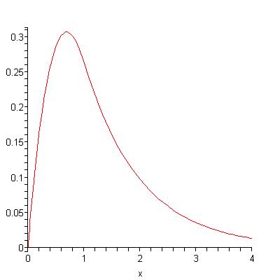
The Oil Shock Model uses a simple rather unbiased multiplier to estimate the oil production response to a discovery input. To demonstrate this, let us take a particular sub-case of the model. If we assume that a discovery immediately becomes extractable, then the multiplying factor for instantaneous production becomes a percentage of what remains. This turns into a damped exponential for a delta discovery (delta meaning a discovery made at a single point in time). In practice, this means that for any particular discovery in the Oil Shock model, we immediately enter a regime of diminishing returns. You can see this in the following plot.


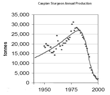
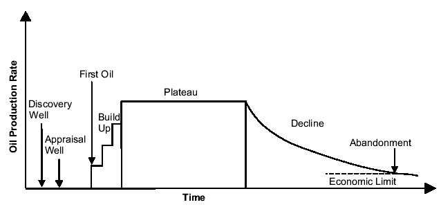
One could argue pragmatically that we rarely enter into an immediately diminishing return regime. In fact, we have all seen the classical regime of an oil bearing region --- this often features an early constant plateau, followed by a drop-off after several years. We usually take this to mean that the oil producers deliberately decide to maintain a constant production rate until the wells no longer produce, in which case we then enter the damped downslope. Or else this could imply that the oil pressure maintains a certain level and the producers extract at the naturally established equilibrium. In fact, the reason that I chose the damped exponential for the Oil Shock model has nothing to do with the intricacies of production; instead it really has to do with the statistics of a spread or range of oil producing wells and regions. The unbiased multiplier really comes from the fact that bigger oil discoveries produce proportionately more oil than smaller oil discoveries, which naturally have less oil to offer. This model becomes nothing more or less than an unbiased statistical estimator for a collection of oil-bearing regions. In other words, the statistics of the collective reduces to a single instance of an average well if we want to think it through from a macro to a micro-perspective. So as a large discovered region starts to deplete, it tends to look statistically more and more like a small producing region, and therefore the fractional extraction estimator kicks in.

With all that said, I can come up with a simple discovery model that matches the behavior of the early plateau observations. We still assume the fractional extraction estimator, but we add in the important factor of reserve growth. Consider the following figure, which features an initial delta discovery at year 1, followed by a series of reserve growth additions of 10% of the initial value over the next 10 years. After that point the reserve growth additions essentially drop to zero.
Next consider that the the extraction essentially scales to the amount of reserve available, and so we set the extraction rate arbitrarily to 10% of the remaining reserve, calculated yearly. (The choice of 10% is critical if you do the math, explained below [1]) Therefore, for a discovery profile that looks like an initial delta function followed by a fixed duration reserve growth period, for the appropriate extraction rate we can come up with the classical micro-production profile.
Wonder of wonders, we see that this micro-model approximates the classical observation of the early plateau followed by a damped exponential. Not coincidentally, the plateau lasts for the same 10 years that the reserve growth takes place in. Rather obviously, we can intuit that this particular plateau maintains itself solely by reserve growth additions. So as the diminishing returns kick in from the initial delta, the reserve growth additions continuously compensate for this loss of production level, as long as the reserve growth maintains itself. After this, the diminishing returns factor eats at whatever reserves we have left, with no additional reserve growth to compensate for it. Voila, and we have a practical model of the classical regime based on the Oil Shock model.

The troublesome feature of the classic plateau lies in its artifice. The underlying discovery model consists of sharp breaks in the form of discontinuities. These manifest themselves in discontinuities in the production model. You see that in the kick-start to immediate stable production due to a delta function in discovery, and then a sharp change in slope due to the sudden end of reserve growth. I don't think anyone actually believes this and I know that Khebab has the same view as he previews in a comment on TOD:

"Now, if you have additional information (peak date, plateau duration, URR, etc.), you could use a more complex model such as the one used by Robelius in his PhD thesis:

I'm currently working on a more complex model."

So from this figure and discussion, we know we must at least account for the build-up, or what I would call the Maturation phase in the Oil Shock model. (The Oil Shock model also considers the Discovery phase and Construction phase but we can ignore these for the purposes of this discussion) This next figure from Khebab aggregates a bunch of these plateau-shaped production profiles from the UK and Norway (where the individual governments' requires close accounting of production levels from the field owners) : 
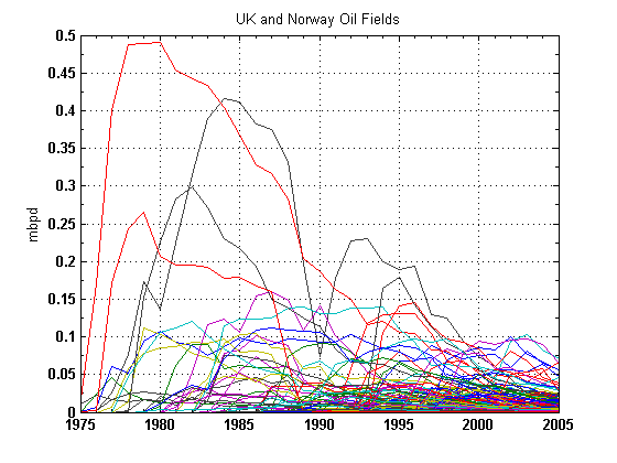
Even though the figure looks busy, note that almost all the profiles show the build-up phase fairly clearly. You can also observe that very few show a stable plateau, instead they mostly show a rounded peak followed by a decline. The asymmetry shows longer tails in the decline than the upward ramp during the build-up phase.

I contend that the Dispersive Discovery model of reserve growth entered into the Oil Shock model can handily generate these kinds of profiles.

The Idea of Shocklets

Khebab has investigated the idea of using loglets (similar to wavelets) in understanding and fitting to multiple-peak oil production profiles. He also used characteristics of the loglet to construct the HSM (and I safely assume his more complex model he hinted at above). As the basic premise behind these "X-let" transforms you find a set of sample signals that when scaled and shifted provides a match to the profile of, say, an oil production curve under examination or some other temporal wave-form. The Oil Shock Model does not differ much in this regard; this salient connection just gets buried in the details of the math [2].

So I suggest that we can visualize the characteristic oil shock model profile by constructing a set of "shocklets" based on the response from a discovery profile input stimulus. The shocklets themselves become micro-economic analogies to the macro view. The math essentially remains the same -- we just use a different prism to view the underlying mechanism.

At the beginning of this discussion, we essentially verified the premise of shocklets by mimicing the plateau regime via a simple discovery/reserve/extraction shock model. That gave us the classical "flat-topped" or plateaued production profile. To modulate the discontinuities and flatness, we use the technique of convolution to combine the damped exponential extraction phase with a modeled maturation phase. The basic oil shock model proposed a simple maturation model that featured a damped exponential density of times; this described the situation of frequent fast maturities with a tail distribution of slower times over a range of production regions.

The exponential with exponential convolution gives the following "shocklet" (with both maturation and extraction characteristic times set to 10 years). Note the build-up phase generated by the maturation element of the model, with very little indication of an extended plateau. (Bentley has a recent TOD post up where he draws a heuristic with a similar shape without providing a basis for its formulation, see the figure to the right)
Now, with a recently established reserve growth model, we can replace the maturation curve with the empirically established reserve growth curve. I make the equivalence between a maturation process and reserve growth additions simply because I contend that extraction decisions get based primarily by how how much reserve the oil producers think lies under the ground -- other maturation effects we can estimate as second-order effects. This essentially makes the connection to and unifies with Khebab's deconvolution approach from backdated discoveries, where he applies Arrington's reserve growth heuristic to the oil shock model and its hybrid HSM. The key idea from Khebab remains the use of the best reserve growth model that we have available, because this provides the most accurate extrapolation for future production.

We start with a general reserve growth curve L2/(L+Time)2 derived from the Dispersive Discovery model. The following figure looks a lot like an exponential (the characteristic time for this is also 10 years) but the DD reserve growth has a sharper initial peak and a thicker longer tail. Compare this to the artificially finite reserve growth profile used to generate the idealized plateau production profile at the beginning of this post.
The shocklet for the DD reserve growth model looks like the following profile in the figure below. Note the build-up time roughly equates with the exponential maturation version, but the realistic reserve growth model gives a much thicker tail. This matches expectations for oil production in places such as the USA lower-48 where regions have longer lifetimes, at least partially explained by the "enigmatic" reserve growth empirically observed through the years. The lack of a long flat plateau essentially occurs due to the dynamics of reserve growth; nature rarely compensates a diminishing return with a precisely balanced and equivalent reserve growth addition. And this matches many of the empirically observed production profiles. The perfectly flat plateau does exist in the real world but the frequent observation of a reserve growth shocklet shape makes it much more useful for general modeling and simulation (the two parameters for characterizing the shape, i.e. an extraction rate and a reserve growth time constant, makes it ultimately very simple and compact as well).
The mantra of the Oil Shock Model still holds -- every year we always extract a fraction of what we think lies underground. The role of reserve growth acts to provide a long-term incentive to keep pumping the oil out of certain regions. As the estimates for additional reserve keep creeping up over time, a fraction of the oil consistently remains available. And by introducing the concept of shocklets, we essentially provide a different perspective on the utility of the Oil Shock Model.


[1]
The solution to the delta plus finite constant reserve shock model is this set of equations:
Po(t) = k e-kt -- production from initial delta, for all t
P1(t) = C (1 - e-kt) -- production from reserve, for t <>
P2(t) = C e-kt (ekT - 1) -- production from reserve, for t > T
Where C is the magnitude of the yearly reserve growth, k is the extraction rate, and T is the duration of reserve growth. Clearly the P0 and P1 terms cancel for the choice of k=C. This will force P0+P1 to maintain a constant level for tT, the curve enters the damped exponential regime.

[2]
Shifting, scaling, and then accumulating many of these sampled waveforms in certain cases emulates the concept of convolution against an input stimulus. For a discovery stimulus, this relates directly to the Oil Shock Model.

Monday, August 18, 2008

Pipes and the Oil Shock Model

No one outside of engineering seems to understand the usefulness of mathematical convolution. To me, it seems a natural operation, as obvious as other more well known statistical operators such as auto-correlation. Yet, you can't find convolution listed in the @function list of a spreadsheet program such as M$ Excel. I have an interest in this because convolution remains at the heart of the Oil Shock Model.

The shock model essentially expresses an oil production curve as a series of temporal convolution operators acting on an initial oil discovery stimulus profile. Each convolution corresponds to a phase of the lifetime of an average discovery, expressed probabilistically to account for the spread in potential outcomes. So that the original discovery profile gets convolved initially by a damped exponential representing the range in fallow times. This output gets followed by a convolution of another profile representing the range in construction times. In turn, the output of this gets convolved into another range of maturation times and then into the final extraction rate profile.

I had previously posted a full program that internally generated the entire set of convolutions, but I finally relented and decided to simplify the concept and use the idea of data flow and short scripts to perhaps make the concept more accessible (and potentially more flexible). Via UNIX or a Windows command shell, one can use the operating system ideas of pipes and the standard input/output streams to generate a very simple instantiation of the Oil Shock Model in terms of a short script and data files.

The pipes in the title of this post offer both an abstraction as to what occurs in the physical world as well as a useful mathematical abstraction to enable us to solve the shock model.

A typical invocation would look something like this:
cat discover.dat | conv fallow.dat | conv cons.dat | conv mature.dat | conv extract.dat
Each one of the phases uses the standard output of the previous phase as a standard input via the operating system pipe command signified by the vertical bar "|". The term conv refers to a shell script or executable that takes the data piped into it and convolves it with data from a file given by the script's command line argument. The initial cat call reads from the discovery data file and pushes it into the first pipe.

In terms of a popular scripting language such as Ruby, the conv script looks like this:
# conf.rb: 
# convolution of stdio input array against array from file

def conv(a, b)
length = a.length + b.length
for i in 0..length do
sum = 0.0
i.downto(0) do |j|
sum += a[i-j].to_f * b[j].to_f
end
puts sum
end
end

conv(STDIN.readlines, IO.readlines(ARGV[0]))
The last line essentially calls the defined convolution function with two arrays generated automatically by using Ruby's readlines file parsing call. So that for each line in the file, representing a year's worth of data, an array is generated both for the standard input data stream, as well as the command line file's data. In other words, "a=the input data" and "b=the convolution data".

Operationally, to call this file using the Ruby interpreter, one has to invoke it with something akin to "ruby conv.rb file.dat". And the data in each of the profiles has to contain enough entries to cover the range of years that you desire to generate a production profile for. The convolution function takes care of the ranges automatically (i.e. the full convolution generates a range that covers the sum of the individual time ranges).

A typical data file for something with a 10 year damped normalized exponential profile would look like:
0.1
0.09048
0.08187
0.07408
....
The ... would go on for N number of lines corresponding to N years. Of course, the data files themselves we can easily generate through other tiny scripts. The UNIX shell has a command called the back-tick "`" which when invoked within the command-line can generate a script call in-place. This means that we have many convenient ways, including providing a lambda function to Ruby itself, to generate the data profiles needed by the convolution operator.

In general, I find nothing really complicated about the convolution operation and find it really a shame that we don't have this functionality built into the set of standard spreadsheet operators. So even though this alternative pipe approach looks incredibly simple in principle, enough people stay away from the command line that it will never achieve the popularity of a spreadsheet formulation. Something like Matlab of course has the convolution operator built-in but it costs big coin and caters to the engineering crowd (of course). Alas, for the moment we will have to satisfy ourselves with pipes.

Update:
I should have added the Shock function to the list of scripts. It essentially acts the same as a convolution, but since it relies on perturbations to a Markov (memoryless) process, we can only add it to the end of the sequence of convolutions. The file it works with contains a list of fractional extraction rates (acting proportionally to the current reserve) matched to the years since the first discovery occurred. For a stationary process, these rates stay relatively constant from year-to-year, but due to the possibility of global events, these rates can suddenly change, leading to sudden blips and dips in yearly production numbers.
The Shock script:

# shock.rb:
# Markov extraction of stdio data using perturbed rates from file

def shock(a, b)
length = b.length
temp = 0.0
for i in 0..length do
output = (a[i].to_f + temp) * b[i].to_f
temp = (a[i].to_f + temp) * (1.0 - b[i].to_f)
puts output
end
end

shock(STDIN.readlines, IO.readlines(ARGV[0]))

The extraction rate file would look like this:
0.1
0.1
0.1
0.12
0.1
....
The fourth entry shows a 20% upward bump in the extraction rate. The complete shock model invocation would thus look like this:
cat discover.dat | conv fallow.dat | conv cons.dat | conv mature.dat | shock rate.dat


Update 2:
The following script takes the standard input and applies a constant extraction rate to the accumulated reserve data. Notice how the convolution simplifies given a Markov approximation.
The un-Shocked script:

# Markov of input array against arg value

def exp(a, b)
length = a.length
temp = 0.0
for i in 0..length do
output = (a[i].to_f + temp) * b
temp = (a[i].to_f + temp) * (1.0 - b)
puts output
end
end

exp(STDIN.readlines, ARGV[0].to_f)
This becomes a "shock"-less model and gets invoked as "ruby exp.rb 0.1", where the argument becomes a single floating-point value instead of a file. The extraction extends for as long as the input data sustains itself, which means that you need to extrapolate the input data if you want to better extrapolate into the future. I suggest this as a useful technique for every one of the scripts.

All of these scripts generate a granularity of only one year so don't expect great results if the rates have time constants that get too close to one year. I would suggest that switching over to a smaller granularity than a year in this case; you just have to remember that the resultant output data will have this same granularity.

Saturday, August 16, 2008

General Dispersive Discovery : The Laplace Transform Technique

It turns out that the generalized Dispersive Discovery model fits into a canonical mathematical form that makes it very accessible to all sorts of additional analysis. Much of the basis of this formulation came from a comment discussion started by Vitalis. I said in the comments that the canonical end result turns into the Laplace transform of the underling container volume density. The various densities include an exponential damping (e.e. more finds near the surface), a point value (corresponding to a seam at a finite depth), a uniform density abruptly ending at a fixed depth, and combinations of the above.

The following derivation goes through the steps in casting the dispersive discovery equations into a Laplace transform. The s variable in Laplace parlance takes the form of the reciprocal of the dispersed depth, 1/lambda. The basic idea again assumes that we search through the probability space of container densities, and accumulate discoveries proportional to the total size searched. The search depths themselves get dispersed so that values exceeding the cross-section of the container density random variable x with the largest of the search variables h get weighted as a potential find. In terms of the math, this shows up as a conditional probability in the 3rd equation, and due to the simplification of the inner integral, it turns into a Laplace transform as shown in the 4th equation.

The fun starts when we realize that the container function f(x) becomes the target of the Laplace transform. Hence, for any f(x) that we can dream up, we can short-circuit much of the additional heavy-duty math derivation by checking first to see if we can find an entry in any of the commonly available Laplace transform tables.

In the square bracketed terms shown after the derivation, I provide a few selected transforms giving a range of shapes for the cumulative discovery function, U-bar. Remember that we still need to substitute the lambda term with a realistic time dependent form. In the case of substituting an exponential growth term for an exponentially distributed container, lambda ~ exp(kt), the first example turns directly into the legendary Logistic sigmoid function that we demonstrated previously.

The second example provides some needed intuition how this all works out. A point container describes something akin to a seam of oil found at a finite depth L0 below the surface. Note that it takes much longer for the dispersive search to probabilistically "reach" this quantity of oil as shown in the following figure. Only an infinitesimal fraction of the fast dispersive searches will reach this point initially as it takes a while for the bulk of the searches to approach the average depth of the seam. I find it fascinating how the math reveals the probability aspects so clearly while we need much hand-waving and subjective reasoning to convince a lay-person that this type of behavior could actually occur.


The 3rd example describes the original motivator for the Dispersive Discovery model, that of a rectangular or uniform density. I used the classical engineering unit-step impulse function u(x) to describe the rectangular density. As a a sanity check, the lookup in the Laplace transform table matches exactly what I derived previously in a non-generalized form, i.e. without the benefit of the transform.

Khebab also suggests that an oil window "sweet spot" likely exists in the real world, which would correspond to a container density function somewhere in between the "seam" container and the other two examples. I suggest two alternatives that would work (and would conveniently provide straightforward analytical Laplace transforms). The first would involve a more narrow uniform distribution that would look similar to the 3rd transform. The second would use a higher order exponential, such as a gamma density that would appear similar to the 1st transform example (see table entry 2d in the Wikipedia Laplace transform table):

Interestingly, this function, under an exponentially increasing search rate will look like a Logistic sigmoid cumulative raised to the nth power, where n is the order of the gamma density! I do wonder if any oil depletion analysts have ever empirically observed such a shape ? (hint, hint, this may require a TOD re-posting)

Monday, August 11, 2008

Examples of Non-Dispersive Peak

From a post on TOD concerning the observation of a Peak Caviar effect,