Petroleum Engineering

With all the discussion on the Gulf Oil disaster going on, lots of petroleum engineers and others from the oil industry have pitched in with their opinions. In which case we can see exactly what they think of their profession.

One commenter, an authority on reservoir engineering apparently had this to say about Peak Oil:

We understand how our business works, certainly. Guys like us, (those IN THE KNOW) have been declaring the end of oil since at least 1886. In Pittsburgh to be specific. Can't say we didn't give the rest of you noobs plenty of warning.

So let me understand this statement. Oil industry types apparently have always known that the end of oil would occur since day one. I wonder why no one thought to just ask them? How did we miss that one?

This same fellow has huge problems with my analysis, because he thinks that what I do amounts to "curve fitting".

I mean seriously, who else would confuse curve fitting with knowledge?

In truth, most of the forecasters who point to continually increasing oil production well into the future base their projections on very little real knowledge. They actually practice curve fitting, i.e. fitting a curve to the production level that we need, because they have no other justification for a realistic outlook.

Bayesian analysis works by using past knowledge to predict future outcomes. We have so much knowledge about previous discoveries, reserve growth mechanisms, and extraction rates that our ability to predict should work very effectively ... if we would just start universally using this kind of approach. The other benefit is that the analysis keeps on getting better and better with time due to the Bayesian updating process. The mathematician Laplace first applied this powerful mode of probabilistic reasoning in the late 1700's to real problems, but we still have holdouts in various disciplines. To top it off, if you have a real model underneath the knowledge, it makes the forecasting that much more powerful.

Let them get through diffy-q, I suppose the only other gang besides engineers forced through that one are the more mathematically inclined....and they are mostly jealous because their theoretical skills don't translate into income very well.

Common knowledge in college that students that went into geology, civil, and petroleum engineering didn't want to get stick in a desk job. Lots of them could not imagine being sedentary for 8 hours a day.

Hubbert peak in Five Easy Pieces

Based on the increase in spill rate from the leaking Gulf of Mexico oil well, HO at TheOilDrum.com suggested a potential explanation. His post essentially argued that sand particles acting as a strong abrasive driven along by the already high velocity stream of escaping oil leads to increasing in the channeling and thus an even faster leak rate.

HO described a process known as CHOPS (Cold Heavy Oil Production with Sand) which can enlarge a well's streaming throughput by promoting the formation of heavily eroded channels. The TOD post provided the following picture of the possible outcome of the behavior.
Note that the lower curve shows the typical output from a throttled flow. Above that curve, the modulated line shows the results of an accelerated extraction -- note that a peak actually appears which pinpoints the maximum flow rate. In terms of the oil spill, we don't want this behavior because it gives us less time to fix or relieve the problem well. Yet, ordinarily we want this same behavior -- that of fast extraction -- in practical situations because we want and need the oil right now! (so that oil companies can make money, of course)

Which leads me to formulating the following very simple but physically correct model of Hubbert's Peak. You won't find this anywhere else, because this derivation does not jive with how geologists think about oil extraction. They get many of the pieces but they never put them all together.

I will offer up a derivation for this behavior leading to a Hubbert Peak in 5 easy pieces.

Piece 1. The standard assumption of draw-down from a reservoir results in an exponential decline over time. You can consider that the exponential shape results from a law of diminishing returns; in that a constant amount proportional to the remainder draws down per unit time. Or you can say that a maximum entropy range of extraction rates gets applied to the volume. A proportional extraction rate that we call R defines the mean and U₀ is the reservoir size. U(t) gives us the cumulative reserve.

U(t) = U₀*exp(-R*t)

Piece 2. Next, we realize that we have uncertainty over the size of the reservoir; the U₀ we have defined actually only serves as an estimate of the size. This means we have an uncertainty over the rate of proportional extraction as well. This turns into a form of hyperbolic discounting and the cumulative draw-down actually looks like this.

U(t) = U₀ / (1+R*t)

Note the fat-tail.

Piece 3. Next we assert that the constant but uncertain proportional extraction rate undergoes an acceleration starting from the original value, R(t) = R₀ + k*t. This acceleration equates to Newton's law, first-order with time. Then the instantaneous absolute rate of extraction from the remaining reservoir looks like:

RateOfExtraction(t) = -dU(t)/dt = U₀*(R₀ + k*t)/(1+R₀*t+k*t²/2)²

For R₀=0.5 and k=2, it results in this shape

This curve we can scale and overlay on top of the CHOPS curve to validate our thought process.

Piece 4. Over a larger set of reservoirs that experience a technical improvement over time, we can assume that the proportional extraction rate can accelerate even more strongly over time, R(t)=C*exp(k*t). This gives us a Moore's law form of acceleration, doubling every set number of years. Then

RateOfExtraction(t) = -dU(t)/dt = U₀ * R(t) / (1+integral(R(t)dt))²

= U₀*C*exp(k*t)/(1+C/k*(exp(k*t)-1))²

For a small starting rate, the acceleration further accentuates the subtle peak that we observe in piece 3 and it turns into a full-fledged symmetric peak as shown in the next figure:

Piece 5. Congratulations. You haven't broken any rules and you have just derived the famed Hubbert Peak, also known as the Logistic Sigmoid function.


Some Backstory
An alternate derivation exists for the corresponding discovery peak, which I call Dispersive Discovery. There, the uncertainty involves how much volume gets explored and at what rate, otherwise the math turns out exactly the same. Both derivations result from an assumed finite constraint but uncertainty in both rates and subvolumes. The only problem with using the Hubbert peak derivation for extraction is that it premises that each extraction rate started at the same time (globally this would be 1858). We know that this has not happened for global production, as extraction can only start after a discovery, and then some variable hold time. By using dispersive discovery, we get a larger spread in start years, and then The Oil Shock model generates the extraction curve. In general, if the discovery peak precedes the oil production peak by a number of years, I would use Dispersive Discovery, but if the two coincide, then extraction tracks discovery and it doesn't really matter how you interpret the rates. This explains why this particular derivation works well for more localized production areas that have seen significant technology changes. In contrast, the technology of discovery has undergone tremendous technology changes over the years, so that dispersive discovery works very well in terms of global modeling. This is actually not much of a caveat, as the more ways that you can find the same result, the more confidence you have that you have remained on the right track.

The current derivation also points out the huge hole in the technique known as Hubbert Linearization (HL). As defined, HL derives from the observation that

dU(t)/dt = U(t)*(U₀-U(t))

Yet this only works for the one case where we can define R(t) as an exponential function, that of piece 4. The formula does not work for either piece 1, 2, or 3. Therefore, HL only serves as a curious mathematical identity for that one exponential case, which we know does not always occur.

The actual "WebHub" Linearization takes the following form:

dU(t)/dt = -U₀ * R(t) / (1+integral(R(t)dt))²

This may not prove as handy as HL perhaps, but it has the benefit of correctness, and it works well for certain cases.

Like me, Robert Rapier has railed against the inadequacy of HL and this may take up the slack.

GOM Reservoir Size Distributions

Question:

BigMoose on June 14, 2010 - 6:26pm Permalink | Subthread | Parent | Parent subthread | Comments top

I have heard many unofficial estimates of the magnitude of oil in this formation... 2nd largest in America, 2nd largest in the world...

Does anyone have a credible estimate on the formation reserves?

Some historical data available from the MMS.
http://www.gomr.mms.gov/PDFs/2009/2009-064.pdf

On the basis of proved oil, for 8,014 proved undersaturated oil reservoirs, the median is 0.3 MMbbl, the mean is 1.8 MMbbl.

Peak Oil theory (Entropic Dispersive Aggregation) says the cumulative size distribution of reservoirs (ranked small to large) goes as P(Size)=1/(1+0.3/Size) if we assume a median of 0.3. It doesn't quite follow this exactly because infinite sized reservoirs can not exist.

If you want the raw data it is here:
file:///G:/RE/Shared/EOGR%20Report/2008-034%20Estimated%20Oil%20and%20Ga...

Sorry, that was a joke, the MMS puts the information on a public web server, and the data is retrieved as a local filesystem URL?
http://www.gomr.mms.gov/homepg/pubinfo/freeasci/geologic/estimated2006.html

I placed whatever data I could get into Google Docs, and placed theory next to it.

The MMS is to be split into 3 agencies apparently. Throughout their history, they failed in doing any kind of useful depletion analysis in the GOM. Anyone can collect data; interpreting it is the challenging part.

The Mentaculus

• Update: Here is a real-life crazy Mentaculus man ⇦ Paul Vaughan is Arthur.

I saw the Coen brothers movie "A Serious Man" a few months ago. A definite period piece from the 1960's, it contrasted two scientists, one an academic and one a hapless amateur. The main protagonist, Larry Gopnick, a physics professor at what looks like a small liberal arts school in the Twin Cities (Macalester, Hamline maybe?), spends time teaching his students what look like elaborate mathematical derivations on a huge chalkboard. He has trouble dealing with some of his students on occasion:

Clive Park: Yes, but this is not just. I was unaware to be examined on the mathematics.
Larry Gopnik: Well, you can't do physics without mathematics, really, can you?
Clive Park: If I receive failing grade I lose my scholarship, and feel shame. I understand the physics. I understand the dead cat.
Larry Gopnik: You understand the dead cat? But... you... you can't really understand the physics without understanding the math. The math tells how it really works. That's the real thing; the stories I give you in class are just illustrative; they're like, fables, say, to help give you a picture. An imperfect model. I mean - even I don't understand the dead cat. The math is how it really works.

His academic colleagues want Professor Gopnick to publish articles at some point (with the implicit threat of not getting tenure). Gopnick's main problem lies in his rationality:

But his rigid framing of a cause-and-effect universe makes him indignant about lack of apparent cause ...

Gopnick's brother, the minor character of Uncle Arthur, takes the role of an almost savant numerologist, busy at work on a treatise called The Mentaculus. Filled with dense illustrations and symbology, it apparently functions as a "probability map" in what appears to spell out a Theory of Everything. It also apparently works to some extent:

We might guess that it makes no sense, but Arthur's "system" apparently "works" as intended, and he applies it to winning at back room card games.

Based on the events that eventually transpire, the theme of the movie essentially says that if you seek rationality, you will ultimately only land on random chance.

I consider myself a "serious man" as well. But do I have a variation of The Mentaculous buried in the contents of this blog?

I tried to make a probability map of all the applications and blog links that I have worked on relating to what I call entropic dispersion in the following table [full HTML]:



The math is how it really works. Perhaps I should publish. Yet blogging is too much fun. Perhaps I need to take a canoe trip.

---

Good reads describing The Mentaculus of probability and statistics

1. "Dawning of the Age of Stochasticity", David Mumford

   From its shady beginnings devising gambling strategies and counting corpses in medieval London, probability theory and statistical inference now emerge as better foundations for scientific models, especially those of the process of thinking and as essential ingredients of theoretical mathematics, even the foundations of mathematics itself.

2. "Probability Theory: The Logic of Science", Edwin T. Jaynes
   

   Our theme is simply: probability theory as extended logic. The ‘new’ perception amounts to the recognition that the mathematical rules of probability theory are not merely rules for calculating frequencies of ‘random variables'; they are also the unique consistent rules for conducting inference(i.e. plausible reasoning) of any kind. and we shall apply them in full generality to that end.

3. "On Thinking Probabilistically", M.E. McIntyre
4. "The Black Swan" and "Fooled by Chance", N.N. Taleb

Worst Book on Oil Crisis Written Yet

Former USGS staffer Steven Gorelick has written a book called "Oil Panic and the Global Crisis: Predictions and Myths". It has to rank as the worst of the neo-cornucopian books out there simply because it actually spreads myths instead of deeming to correct them, as the title implies.

The author acts the role of a somewhat neutral bystander and balanced pseudo-journalist, never giving the appearance of a rabid oil cornucopian, yet slipping in so many groaners that he basically gives away his not-so-hidden agenda. From a scientific context, providing both sides of the story makes no sense when the objective is truth rather than balanced reporting. Excerpts of the book would fit right into a Fox news piece.

To give a taste of how little original research that Gorelick has actually performed and how much he relies on other cornucopians, consider the passage wherein he references geology professor Larry Cathless. On page 128, Gorelick quotes Cathles as saying that we may find as much as "1 trillion barrels of oil and gas in just a portion of the gulf oil sediments".

I found the original statement by Cathles here:

Cathles and his team estimate that in a study area of about 9,600 square miles off the coast of Louisiana, source rocks a dozen kilometers down have generated as much as 184 billion tons of oil and gas — about 1,000 billion barrels of oil and gas equivalent. "That's 30 percent more than we humans have consumed over the entire petroleum era," Cathles says. "And that's just this one little postage stamp area; if this is going on worldwide, then there's a lot of hydrocarbons venting out."

Although not directly implicated as an abiotic oil advocate (unlike his late Cornell University colleague Thomas Gold), former Chevron employee Cathles has close ties to the largely mythical Eugene Island story. Several years ago new discoveries from the previously tapped-out Eugene area had people's hopes up that somehow oil reservoirs could go through a near real-time "replenishment".

"We're dealing with this giant flow-through system where the hydrocarbons are generating now, moving through the overlying strata now, building the reservoirs now and spilling out into the ocean now," Cathles says.

Well, as it turned out, the Eugene Island secondary production turned out just a blip on the radar screen, yet Cathles still gets a mention as a credible source? (Think about it, if this turned out true, then the recent Gulf Oil spill could allow a never-ending release of hydrocarbons from beneath the waters, as this urban legend gets repeated still. How embarrassingly timely for Gorelick.).

Elsewhere, the book becomes safe pablum for a narrowly defined audience. Note the limited depth of Gorelick's analysis and the intentional dumbing down in his writing:

Hubbert used a straightforward formula that yields the curve as illustrated in Figure 1.2. The logistic-curve formula is a simple expression with three adjustable parameters (mathematical knobs) that control the slope, peak, height and time of peak

Now you see what happens when an author keeps it too simple. He ends up never explaining anything about the logistic, apart from providing the functional form in a footnote, and makes it worse by calling the parameters "mathematical knobs". That essentially gives a flavor of the depth of the mathematics.

Gorelick has an entire chapter called "Counter-Arguments to Imminent Oil Depletion". Notwithstanding that oil depletion is imminent by definition (it certainly does not regenerate contrary to the implications), this chapter contains some of the most unscientific assertions that I have come across. Consider this bullet point coming from Gorelick:

- The world has never run out of any significant globally traded, non-renewable Earth resource.

This false equivalency comes somewhere from the list of logical fallacies. I find it bizarre that a reputable scientist would appeal to this kind of argument. Further he bullet points:

- The trends in production of global oil and natural gas have not declined as predicted.

I call a strawman fallacy as no one has really come up with a formal theory for depletion. Instead every oil prediction that I have seen has relied on some sort of ad hoc analysis via heuristics. So to imply that something has not followed as predicted does not prove anything. As I have said before, heuristics do not substitute for theory and Gorelick unfortunately has not contributed any research of his own.

I listed only 2 of the 21 bullet pointed counter-arguments that Gorelick concludes the chapter with. I can understand the need for these bullet points if he wanted to act like an objective journalist wanting to tell both sides of the story. Yet we have all learned from Krugman that real science does not scream headlines that say "Shape of Earth--Views Differ". A scientist should dig deep and try to come up with a model or theory that would confirm or rebut the empirical evidence. You just don't rely on tired worn-out assertions (the world has never run out of a resource, predictions have not come true, etc) from the cornucopian right, put them in a book and consider this an advancement of knowledge.

The book industry likely published Oil Panic because it does not even remotely challenge business as usual and actually condones the cornucopian viewpoint.

End of book review.

---

Musings

Since Gorelick has propagated half-truths and not resolved any myths at all in the oil depletion realm, I figured I would return the favor in his own research area. From his CV, the "honored and awarded" Gorelick moved on from the USGS and became a professor of hydrogeology and part of the Environmental Earth System Science department at Stanford University. If he can write a book on peak oil and turn back progress on understanding oil depletion, I can opine on hydrogeology.

From his research papers, Gorelick claims to understand how to model principles of hydrogeology and presumably knows about breakthrough curves. It turns out that most of the dispersive transport involved in hydrology applications hinges on some very simple overriding principles. These principles are so obvious to me that I don't understand why the brilliant scientific minds in geology have not figured this out. Consider that Gorelick has expertise in "multiple-rate mass transfer" which I associate this with the simple idea of dispersion applied to material transport. I actually ran across Gorelick's work prior to reviewing his book because of my studies of generalized dispersive transport.

As Gorelick should know, all processes do not proceed at the same rate, and this includes variations in oil discovery rates around the world. This leads directly to the fat-tail effects that I see in oil reserves and to the fat-tails that Gorelick observes in solute transport in his groundwater contamination studies. Not all solute diffuses and drifts at the same rate, so that scientists see these long tails. How Gorelick can publish research on groundwater rates, but see no analogy to the larger issue of oil extraction seems such a waste of intellectual potential.

Should Gorelick ever read this review, I challenge him to read my work on dispersion and the math behind depletion of oil. These models come from solid math and probability underpinnings and simple physical first principles, and lead to the kind of insight that we all need to make sense of our fossil fuel energy situation.

Oil Discovery Simulation Reality

I should have run this particular simulation long ago. In this exercise, I essentially partitioned the Dispersive Discovery model into a bunch of subvolumes. Each subvolume belongs to a specific prospecting entity, which I have given a short alias. The simulation assigns each one of the entities a random search rate and each one of the subvolumes also has a randomly sized value. The physical analogy equates to the prospector (i.e. the entity is an owner, leaser, company, nation, etc.) given their own subvolume (geographic location) to explore for oil. When they exhaustively search that subvolume, they end up with a cumulative amount of oil. The abstraction for subvolumes allows for the random sizing to directly translate to a proportional amount of oil. In general, bigger subvolumes equates to more oil but this does not have to hold, since the random rates blur this distinction.

Removing the technical mumbo-jumbo, the previous paragraph describes quite simply the context for the dispersive discovery model. Nothing about this description can possibly get misinterpreted as it essentially describes the process of a bunch of people systematically searching through a haystack for needles. Each person has varying ability and owns a varying size to search through, which essentially describes the process of dispersion.

The random number distributions derive from a mean search rate and a mean subvolume based on the principle of maximum entropy (MaxEnt). The number of subvolumes multiplied by the mean subvolume generates an ultimately recoverable resource (URR) total. By building a Monte Carlo simulation of this model, we can see how the discovery process plays out for randomly chosen configurations.

When the simulation executes, the search rates accelerate in unison so that the variance remains the same, maintaining MaxEnt of the aggregate. If I choose an exponential acceleration, the result turns precisely into the Logistic sigmoid, also known as the classic Hubbert Curve..

The entire simulation exists on a Google spreadsheet. Each row corresponds to a prospecting entity/subvolume pairing. The first two cells provide a random starting rate and a randomly assigned subvolume. As you move left to right across the row, you see the fraction of the subvolume searched increase in an accelerating fashion with respect to time. The exponential growth factor resides in cell A2. At some point in time, the accelerating search volume meets the fixed volume constraint and the number stops increasing. At that moment, the prospector has effectively finished his search. That subvolume has essentially ceased to yield newly discovered oil.

I reserve the 4th row for the summed values, the 3rd line generates the time derivative which plots out as a yearly discovery. The simulation "runs" one Monte Carlo frame at a time. We essentially see a full snapshot of one sample for about 150 years of dispersive search.

View Google Spreadsheet

I associated short names for each of the prospecting entities[1]. As I did not to want to make the spreadsheet too large, I limited it to 250 entities (which pushes Google to the limit for data). This of course introduces some noise fluctuations. The non-noisy solid line displays the analytical solution to the dispersive discovery model, which happens to match the derivative of the Logistic sigmoid.

The most important insight that we get from this exercise has to do with generating a BLINDINGLY SIMPLE explanation for deriving the Logistic behavior that most oil depletion analysts assume to exist, yet have no basis for. For crying out loud, I have seen children's board games with more complicated instructions than what I have given in the above paragraphs. Honestly, if you find someone that can't understand what it is going on from what I have written, don't ask them to play Chutes & Ladders either. Common sense Peak Oil theory ultimately reduces to this basic argument.

Contrast the elegance of the dispersive model with the most common alternative derivation for the logistic peak shape. This involves a completely misguided deterministic model that not surprisingly makes ABSOLUTELY NO SENSE. Whoever originally dreamed up the Verhulst derivation for ecological modeling and decided to apply it to Peak Oil must have consumed large quantities of mind-altering drugs prior to putting pencil to paper.

I also want to point out that what I did has nothing to do with multi-cycle Hubbert modeling which adds even less insight to the fundamental process.

I hope that this exercise helps in understanding the mechanism behind dispersive discovery. Seriously, the big intuitive sticking point that people have with the model has to do with the lack of any feedback mechanism in dispersive discovery. I imagine that engineers and most scientists get so used to seeing the feedback-derived Verhulst and LV equations derive the Logistic that they can't believe a simple and correct formulation actually exists!

In real terms, at some point the oil companies will cease to discover much of anything as they exhaust search possibilities. I suggest that they might want to consider making up for lost profit by licensing the oil discovery board game. This would help explain to their customers the reality of the situation.

UPDATE:
Occasionally Google does an underflow or overflow on some calculations so that the aggregate curve won't plot. The following animated GIF shows a succession of curves:

---

[1] I used shortened versions of TOD commenter names in the spreadsheet to make it a little more entertaining. I probably spent more time on writing the names down and battling the sluggishness of Google spreadsheet than I did on the simulation.

Predictably Unreliable

I wrote about the unpredictably predictable nature of wind power in a few recent posts.

And of course we have watched the unexpected and unpredicted blow-out of the Deepwater Horizon oil well (the ultra-rare 1 out of 30,000 failure according to conventional wisdom) and hoping for the successful deployment of relief wells.

In the wind situation we know that it will work at least part of the time (given sufficient wind power, that is) without knowing precisely when, while in the second case we can only guess when a catastrophe with such safety-critical implications will occur.

We also have the unnerving situation of knowing that something will eventually blow-out, but with uncertain knowledge of exactly when. Take the unpredictability of popcorn popping as a trivial example. We can never predict the time of any particular kernel but we know the vast majority will pop.

In a recent episode that I went through, the specific failure also did not come as a surprise. I had an inkling that an Internet radio that I frequently use would eventually stop working. From everything I had read on-line, my Soundbridge model had a power-supply flaw that would eventually reveal itself as a dead radio. Previous customers had reported the unit would go bad anywhere from immediately after purchase to a few years later. After about 3 years it finally happened to my radio and the failure mode turned out exactly the same as everyone else's -- a blown electrolytic capacitor and a possible burned out diode.

The part obviously blew out because of some heat stress and power dissipation problem, yet like the popcorn popping, my interest lies in the wide range in failure times. The Soundbridge failure in fact looks like the classic Markov process of a constant failure rate per unit time. In a Markov failure process, the number of expected defects reported per day equate proportionally to how many units remain operational. This turns into a flat line when graphed as failure rate versus time. Customers that have purchased Soundbridges will continue to routinely report the failures for the next few years, with fewer and fewer reports as that model becomes obsolete.

Because of the randomness of the failure time, we know that any failures should follow some stochastic principle and likely that entropic effects play into the behavior as well. When the component goes bad, the unit's particular physical state and the state of the environment governs the actual process; engineers call this the physics of failure. Yet, however specific the failure circumstance, the variability in the component's parameter space ultimately sets the variability in the failure time.

So I see another way to look at failure modes. We can either interpret the randomness from the perspective of the component or from the perspective of the user. If the latter, we might expect that someone would abuse the machine more than another customer, and therefore effectively speed up its failure rate. Except for some occasional power-cycling this likely didn't happen with my radio as the clock stays powered in standby most of the time. Further, many people will treat their machine gingerly. So we have a spread in both dimensions of component and environment.

If we look at the randomness from a component quality-control perspective, certainly manufacturing variations and manual assembly plays a role. Upon internal inspection, I noticed the Soundbridge needed lots of manual labor to construct. Someone posting to the online Roku radio forum noticed a manually extended lead connected to a diode on their unit -- not good from a reliability perspective.

So I have a different way of thinking about failures which doesn't always match the conventional wisdom in reliability circles. In certain cases the result derives as expected, but in other cases the result diverges from the textbook solution.

Fixed wear rate, variable critical point: To model this to first-order, we assume a critical-point (cp) in the component that fails and then assume a distribution of the cp value about a mean. Maximum entropy would say that this distribution would approximate an exponential:

p(x) = 1/cp * exp(-x/cp)

The rate at which we approach the variable cp remains constant at R (everyone uses/abuses it at the same rate). Then the cumulative probability of failure is

P(t) = integral of p(x) from x=0 to x=R*t

This invokes the monotonic nature of failures by capturing all the points on the shortest critical path, and anything "longer" than the R*t threshold won't get counted until it fails later on. The solution to this integral becomes the expected rising damped exponential.

P(t) = 1 - exp(-R*t/cp)

Most people will substitute a value of τ for cp/R to make it look like a lifetime. This is the generally accepted form for the expected lifetime of a component to first-order.

P(t) = 1 - exp(-t / τ)

So even though it looks as if we have a distribution of lifetimes, in this situation we actually have as a foundation a distribution in critical points. In other words, I get the correct result but I approach it from a non-conventional angle.

Fixed critical point, variable rate: Now turn this case on its head and say that we have a fixed critical point and we have a maximum entropy variation in rate assuming some mean value, R.

p(r) = 1/R * exp(-r/R)

Then the cumulative integral looks like:

P(t) = integral of p(r) from r=cp/t to r=∞

Note carefully that the critical path in this case captures only the fastest rates and anything slower than the cp/t threshold won't get counted until later.

The result derives to

P(t) = exp(-cp/(R*t))

This has the characteristics of a fat-tail distribution because time goes into the denominator of the exponent, instead of the numerator. Physically, this means that we have very few instantaneously fast rates and many rates proceed slower than the mean.

Variable wear rate, variable critical point: In a sense, the two preceding behaviors act complementary to each other. So we can also derive P(t) for the situation whereby both the rate and critical point vary.

P(t) = integral of P(t | r)*p(r) over all r

This results in the exponential-free cumulative, which has the form of an entroplet.

P(t) = R*t/cp / (1+ R*t/cp) = t/τ/(1+t/τ)

Plotting the three variations side-by-side and assuming that τ=1, we get the following set of cumulative failure distributions. The full variant nestles in between the two other exponential variants, so it retains the character of more early failures (ala the bathtub curve) yet it also shows a fat-tail so that failure-free operation can extend for longer periods of time.

To understand what happens at a more intuitive level we define the fractional failure rate as

F(t) = dP/dt / (1-P(t))

Analysts use this form since it makes it more amenable to predicting failures on populations of parts. The rate then applies only to how many remain in the population, and the ones that have failed drop out of the count.

Only the first case above gives a failure rate that approaches the Markov ideal of constant rate over time. The other two dip below the constant rate of the Markov simply because the fat-tail cumulative requires a finite integrability over the time scale, and so the rates will necessarily stay lower.

Another post gives a full account of what happens when we generalize the first-order linear growth on the rate term, letting R=g(t). The full variant ultimately gives dg/dt / (1+g(t)), so that if g(t) starts rising we get the complete bathtub curve.

If we don't invoke other time dependencies on the rate function g(t), we see how certain systems never show failures after an initial period. Think about it for a moment -- the fat-tails of the variable rate cases push the effective threshold for failure further and further into the future.

In effect, normalizing the failures in this way explains why some components have predictable unreliability, while other components can settle down and seemingly last forever after the initial transient.

I discovered that this paper by Pandey jives with the way I think about the general problem.

Enjoy your popcorn, it should have popped by now.

Reliability of Relief Wells

I have seen much discussion on TOD and elsewhere of the effectiveness of adding relief wells to take the pressure off the failed well in the Gulf. Occasionally I have noticed questions on how one would make a kind of reliability prediction given estimated success/failure probability numbers. This turns into the classic redundant configuration reliability prediction problem.

Initially, for pure success probabilities I wouldn't add time to the equation. In the steady-state we just work with basic probability multiplications. If the probabilities of success rates remain independent of each other, then they form a pattern. Say we have three tries for relief wells, each one having a value between 0 and 1. If all three fail then the whole attempt failed:

P(failure) = P1(failure)*P2(failure)*P3(failure)

and

P(success)=1-P(failure)

so if P1=P2=P3=1-0.7=0.3

then P(failure)=0.027

and P(success)=0.973

With time you need to work from the notion of a deadline, i.e. that no failures occur in a certain amount of time. Otherwise you end up using the fixed probabilities above because you have essentially infinite time to work with.

Apart from end-state failure analysis, you can also do a time-averaged effectiveness, where the rates help you do a trade-off analysis between how long it takes before you fix the problem and how much oil gets released in the meantime. Unfortunately, when you look at the optimization criteria, the only valid optimum in most people's minds is to stop the oil leak as quickly as possible. Otherwise it looks like we play dictator rolling dice (at least IMO that is the political response I predict to get).

Given that political issue, you can create a set of criteria with weights on the probabilities of success, the cost, and on the amount of oil leaked (the first and third as Markov models as a function of time). When you combine the three and look for an optimum, you might get a result that gives you a number of relief wells somewhere between 1 and infinity. The hard part remains establishing the weighting criteria. Place a lower weight on cost and you will definitely lower the number of wells. And that's where the politics plays in again, as many people will suggest that cost does not form a limitation. We also have the possibility of a massive blow-out by adding a botched relief well, but that risk may turn out acceptable.

Below I show a state diagram from a Markov-based reliability model. With the Markov process premise you can specify rates of probability flow between various states and then execute it without having to resort to Monte Carlo.

I made this diagram for 3 relief wells drilled in succession, when one doesn't work, then we start the next. The term B1 is the rate for a failure specified as 0.01 (or 1 in 100 days). B2 is a success rate of 0.02 (or 1 in 50 days). The start state is P1, the success state is P3, and the end failure state is P5.

When I execute this for 200 days, the probability of entering state P5 is 3.5% and it will rise to 3.7% after 1000 days. P3 is 95% after 200 days. The sanity check on this gives a success ratio of about 0.02/(0.01+0.02)=0.666 and from the formula this gives a probability of failure at the end state of (1/3)^3 = 0.037 = 3.7%. This sanity checks with the output after 1000 days.

The Markov model allows you to predict the time dependence of success and failure based on the assumptions of the individual non-redundant failure rates. You can thus work the model as a straightforward reliability prediction. Change the success probabilities to 50% individual success rate and we still only need three relief wells if we want to get to 87.5% . Contrast that to 97% average success rate with 3 wells, if we remain on the optimistic side of 50%. So you can see that our confidence grows with the confidence in the success of the individual wells, which makes intuitive sense.

This particular model assumes a serial succession of relief wells. You can also model relief wells constructed in parallel, which I believe remains the current strategy in the Gulf. Or you can model the initial delay a little better. With the model as described, we have success rates that can occur earlier than perhaps expected. An exponential on the success rate per time provides a distribution where the standard deviation equals the mean, which is the most conservative estimator should you have no idea what the standard deviation is. To generate a model with about half the standard deviation, we can turn the exponential into a gamma. Each relief well spends about half its time in a "build" stage where it experiences neither success or failure. Then the next stage of its life-cycle gets spent in testing for success. See the following chart:

The overall result doesn't differ much from the previous model but you do see a much diminished success rate early on -- which makes the model match reality better.

As another possibility, we can repeat an individual relief well several times, backing up and retrying if the last one doesn't work. That models as a state that directs back on itself, with a rate B4. I won't run this one because I don't know the rates of retries, but the general shape of the of the failure/success curve looks similar.

I'm sure some group of analysts somewhere has worked a similar kind of calculation. Whether it pays off or not for a single case, I can't really say. However, this kind of model effectively describes how the probabilities work out and how you can use a state diagram to keep track of failure and success transitions.

By the way, this same math goes into the Oil Shock Model which I use for oil production prediction. In the oil shock model, transitions describe the rates between oil production life-cycle states, such as construction and maturation and extraction. So both the reliability model and the Oil Shock model derive from probability-based data flow models. This kind of model works very well for oil production because we have a huge number of independently producing regions around the world and the law of large numbers makes the probability projections that much more accurate. As a result, I would put more trust in relying on the results of the oil shock model than predicting the success of the recovery of a single failed deep-water production well. Yet, the relief well redundancy model does help to estimate how many extra relief wells to add and adds some quantitative confidence to one's intuition.

---

Based on the post by Joules Burn (JB) on TOD BP's Deepwater Oil Spill: A Statistical Analysis of How Many Relief Wells Are Needed, I added a few comments:

JB did everything perfectly correctly given the premises. Another way to look at it is that you need to accomplish a sequence of steps, each with a probability rate of entering into the next state. This would simulate the construction of the relief well itself (a sequence of steps). Then you would have a rate into a state where you start testing the well for success. This goes into a state that results in either a success, retry, or failure (the utter failure in JB lingo). The convenient thing is that you can draw the retry as a feedback loop, so the result looks like the following for a single well:


I picked some of the numbers from intuition, but the results have the general shape that JB showed. When you look at a rate like 0.1, inverting it gives a mean transition of 10 days.

This is a state diagram simulation like that used in the Oil Shock model, which I use to project worldwide oil production. I find it interesting to see how well accepted the failure rate approach is for failure analysis, but few seem to accept it for oil depletion analysis. I presume oil depletion is not as mission critical a problem as the Gulf spill is :)

Thermal Entropic Dispersion

As we learn how to extract energy from disordered, entropic systems such as amorphous photovoltaics and wind power, we can really start thinking creatively in terms of our analysis. Most of the conventional thinking goes out the window as considerations of the impact of disorder requires a different mindset.

In a recent post, I solved the Fokker-Planck diffusion/convection equation for disordered systems and demonstrated how well it applied to transport equations; I gave examples for both amorphous silicon photocurrent response and for the breakthrough curve of a solute. Both these systems feature some measurable particle, either a charged particle for a photovoltaic or a traced particle for a dispersing solute.

Similarly, the conduction of heat also follows the Fokker-Planck equation at its most elemental level. In this case, we can monitor the temperature as the heat flows from regions of high temperature to regions of low temperature. In contrast to the particle systems, we do not see a drift component. In a static medium, not abetted by currents (as an example, mobile ground water) or re-radiation, heat energy will only move around by a diffusion-like mechanism.

We can't argue that the flow of heat shows the characteristics of an entropic system -- after all temperature serves as a measure of entropy. However, the way that heat flows in a homogeneous environment suggests more order than you may realize in a practical siuation. In a perfectly uniform medium, we can propose a single diffusion coefficient, D, to describe the flow or flux. A change of units translates this to a thermal conductivity. This value inversely relates to the R-value that most people have familiraity with when it comes to insulation.

For particles in the steady state, we think of Fick's First Law of Diffusion. For heat conduction, the analogy is Fourier's Law. These both rely on the concept of a concentration gradient, and functionally appear the same, only the physical dimensions of the parameters change. Adding the concept of time, you can generalize to the Fokker-Planck equation (i.e Fick's Second Law or the Heat Equation respectively).

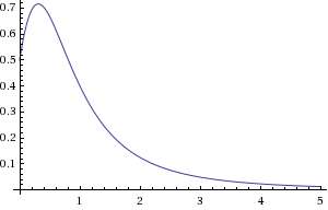
Much as with a particle system, solving the one-dimensional Fokker-Planck equation for a thermal impulse you get a Gaussian packet that widens from the origin as it diffuses outward. See the picture to the right for progressively larger values of time. The cumulative amount collected at some point, x, away from the origin results in a sigmoid-like curve known as an complementery error function or erfc.

Yet in practice we find that a particular medium may show a strong amount of uniformity. For example, earth may contain large rocks or pockets which can radically alter the local diffusivity. Same thing occurs with the insulation in a dwelling; doors and windows will have different thermal conductivity than the walls. The fact that reflecting barriers exist means that the effective thermal conductivity can vary (similarly this arises in variations due to Rayleigh scattering in wind and wireless observations). I see nothing radical about the overall non-uniformity concept, just an acknowledgment that we will quite often see a heterogeneous environment and we should know how to deal with it.

Previously, I solved the FPE for a disordered system assuming both diffusive and drift components. In that solution I assumed a maximum entropy (MaxEnt) distribution for mobilities and then tied diffusivity to mobility via the Einstein relation. The solution simplifies if we remove the mobility drift term and rely only on diffusivity. The cumulative impulse response to a delta-function heat energy flux stimulus then reduces to:

T(x,t) = T1* exp(-x/sqrt(D*t)) + T0

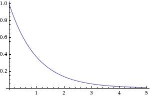
No erfc in this equation (which by the way makes it useful for quick analysis). I show the difference between the two solutions in the graph to the right (for a one-dimensional distance x=1 and a scaled diffusivity of D=1). The uniform diffusivity form (red curve) shows a slightly more pronounced knee as the cumulative increases than the disordered form (blue curve) does. The fixed D also settles to an asymptote more quickly than the MaxEnt disordered D does, which continues to creep upward gradually. In practical terms, this says that things will heat up or slow down more gradually when a variable medium exists between yourself and the external heat source

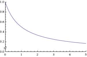
Because of the variations in diffusivity, some of the heat will also arrive a bit more quickly than if we had a uniform diffusivity. See the figure to the right for small times. Overall the differences appear a bit subtle. This has as much to do with the fact that diffusion already implies disorder, while the MaxEnt formulation simply makes the fat-tails fatter. Again it essentially disperses the heat -- some gets to its destination faster and a sizable fraction later.

Which brings up the question of how we can get some direct evidence of this behavior from empirical data. With drift, the dispersion becomes much more obvious, as systems with uniform mobility with little disorder show very distinct knees (ala photocurrent time-of-flight measurements or solute breakthrough curves for uniform materials) . Adding the MaxEnt variation makes the fat-tail behavior very obvious, as you would observe from the anomalous transport behavior in amorphous semiconductors. With diffusion alone, the knee automatically smears, as you can see from the figure to the right for a typical thermal response measurement.

Evidence
Much of the interesting engineering and scientific work in characterizing thermal systems comes out of Europe. This paper investigating earth-based heat exchangers contains an interesting experiment. As a premise, they wrote the following, where incidentally they acknowledge the wide variation in thermal conductivities of soil:

The thermal properties can be estimated using available literature values, but the range of values found in literature for a specific soil type is very wide. Also, the values specific for a certain soil type need to be translated to a value that is representative of the soil profile at the location. The best method is therefore to measure directly the thermal soil properties as well as the properties of the installed heat exchanger.

This test is used to measure with high accuracy:

• The temperature response of the ground to an energy pulse, used to calculate:
  • the effective thermal conductivity of the ground
  • the borehole resistance, depending on factors as the backfill quality and heat exchanger construction
• The average ground temperature and temperature - depth profile.
• Pressure loss of the heat exchanger, at different flows.

The authors of this study show a measurement for the temperature response to a thermal impulse, with the results shown over the course of a couple of days. I placed a solid red and blue line indicating the fit to an entropic model of diffusivity in the figure below. The mean diffusivity comes out to D=1.5/hr (with the red and blue curves +/- 0.1 from this value) assuming an arbitrary measurement point of one unit from the source. This fit works arguably better than a fixed diffusivity as the variable diffusivity shows a quicker rise and a more gradual asymptotic tail to match the data.


The transient thermal response tells us a lot about how fast a natural heat exchanger can react to changing conditions. One of the practical questions concerning their utility arises from how quickly the heat exchange works. Ultimately this has to do with extracting heat from a material showing a natural diffusivity and we have to learn how to deal with that law of nature. Much like we have to acknowledge the entropic variations in wind or cope with variations in CO2 uptake, we have to deal with the variability in the earth if we want to take advantage of our renewable geothermal resources.

Wind Variability in Germany

By adding more data to the post on wind dispersion, we can observe how dispersion in wind speeds has a universal character. I picked up the previous data set from several years worth of output from Ontario. This new set hails from northwest Germany and this site (thanks to globi for the link). The data consists of wind power collected at 15 minute intervals.


Note that the same entropic dispersion holds as for Ontario (see graph to the right). Both curves display the same damped exponential probability distribution function for frequency of wind power (derived from wind speed). We also see the same qualitative cut-out above a certain power or wind energy level. As I said previously, we don't gain much by drawing from these higher power levels as they occur more sporadically than the nominally rated wind speeds at the upper reaches of the curve.

The following figure gives an explanation for the cutout above the "max" wind speed. Globi also provided this PDF from Vestas, a maker of wind turbines. The end of the document has the complete spec.

Power regulation : pitch regulated with variable speed
Operating data
Rated power : 3,000 kW Cut-in wind speed : 3 m/s
Rated wind speed : 12 m/s
Cut-out wind speed : 25 m/s

Too many people get the idea that the sporadic nature of wind confronts us with some kind of "problem". We will have to get used to a different way of thinking about wind. The entropic dispersion of wind acts much like a variation of the Carnot cycle. In the Carnot cycle of engine efficiency, we have to live with a maximum level of energy conversion based on temperature differences of the input and output reservoirs. With wind, the earth's environment and atmosphere provides the temperature differences which leads directly to the variability over time.

Which leads to the fact that WITH WIND POWER, WE CAN ACHIEVE VERY HIGH USAGE EFFICIENCY GIVEN THE ENTROPIC CHARACTERISTICS OF THE WIND. I put this in upper case because it amounts to a law of nature. We need to talk about efficiencies within the constraints of the physical laws just as with the Carnot cycle. We will observe intermittency as a result of entropic dispersion and we have to get used to it. We should not call it a fundamental "problem", as we cannot change the characteristics of entropy (apart from adding energy, and that just moves us back to square one).

Other people would suggest that the fundamental problem with farming derives from the intermittent nature of the rain. With farming, we adapt -- likewise with wind energy. Instead of a problem, we need to call it an opportunity.

---

As a blast from the past check out my expose of the forged video editing by the George Bush marketing team against John Kerry. Wind energy advocates will have to watch out for these tactics as the right-wingers will project and frame any way they can to make wind look like a wimpy exercise designed by the elite for the elite.