Fitting

I went back and looked at the data in my Network Dispersion post from a while ago. At the time I didn't plot it to show the strong power-law characteristics of the dispersive rate formulation, so replotted it here:


This is a simple distributed latency caused by the dispersed network transport rate, where the cumulative P(Time) = exp(-T₀/Time). The derivative is a PDF and this gives the 1/Time² slope shown (adjusted for the log density along the horizontal axis). Some uncertainty exists in the minimum measurable round-trip time at around 1 ms, but the rest of the curve agrees with the simple entropic dispersion -- a slight variation of the basic entroplet in action.

Neater still is the entropic dispersion in daily rainfall data. I happened across research work at the National Center for Atmospheric Research under the title "Extreme Event Density Estimation". The researchers there seem to think the following graph has some mysterious structure. It basically displays a histogram of daily rainfall in January at a station in North Carolina.



On first glance, this data doesn't appear highly dispersed as the tail stays fairly thin, yet take a look at this fit:


You need to understand first that a critical point exists for rain to fall. The volume and density at which nature reaches this critical point has much to do with the rate at which a cloud increases in intensity. If we assume that clouds develop by some sort of preferential attachment, then the uncertainties at which the preferential attachment process increases with time balanced against the uncertainties in the critical point contribute to the entropic dispersion:

p(x) = r/(r+g(x))²

The term g(x) essentially measures the preferential attachment accelerated growth rate:

g(x) = k*(exp(a*x) - 1)

This has the mechanism for preferential attachment since dg/dx = a * (g(x)+k), which describes exponential growth plus a linear term. When plotted, we get the orange curve shown plotted along with the data points, where r=1, a=1/17 years and k=2 (dimensions in mm). Coicidentally, this is actually just the logistic sigmoid function; we never see the characteristic peak or inflection point since it starts off well up the towards the halfway point of the cumulative (see the following graph where I used r=10 to accentuate the sigmoid peak).



In spite of the good fit, this curve has a limited locality: consisting of one rainfall station in North Carolina. What happens when we look at the distribution of rainfall on a global scale?

This poster and slide show attempts an understanding of the distribution via entropy arguments.

The curve below does not work as well for the exponential growth (bright green) but it does work very well for the cubic-quadratic growth model (cumulative growth ~ x⁵, bright turquoise) that I used in my analysis of dispersive discovery of oil reservoirs. (note that this curve is plotted in hydrologist's lingo, where the rate of return in years T equates to a histogram bin. The rate of return analogizes to principle such as the "100 year storm"). The values shown here are in inches of rainfall, not millimeters as in the previous figure.



Since we can expand an exponential in terms of a Taylor series and see a sum of power terms, it makes some sense that the t ⁵ term may emulate the exponential growth (or vice versa), or perhaps generate the limiting trend. Exponential growth eventually moderates and the 5^th power may provide the major effect along the curve over the remainder of the fat tail (note that the power is 5 and not 6 in the cubic-quadratic model because rainfall is measured as a linear measure and growth of water content goes as volumetric density).

As the arguments for oil discovery (uncertain acceleration in technology along an uncertain volume) emulate rain strength (uncertain acceleration in cloud/droplet growth along an uncertain critical volume/density), I consider this a further substantiation of the overall entropic dispersion formulation.

Yet I've got to wonder: do climate scientists think this way? The hydrology researcher Koutsoyiannis, who identified the power-law dependence in the previous figure, seems to have gotten on the right track. His multiple Markov chain remains a bit unwieldy as he can only generate a profile via simulation, yet that may not matter if we can use a power-law argument directly as I did for dispersive discovery. This needs a deeper look as it exposes a few remaining modeling details in a comprehensive theory.

---

Speaking of odd, why do these rather simple arguments always seem to work so well, and, extending that, could dispersion work everywhere? The odd thing is that the odds function may hold a bit of the key. Everyone seems to understand how gambling works, particularly in the form of sports betting, where just about any lame-brained man-off-the-street comprehends how the odds function works. Odds against for some competitor to win is essentially cast in terms of the probability P:

Odds = (1-P)/P

When plotted the odds distribution looks like the following curve:


Which then looks exactly like the rank histogram of any scaled entropic dispersion process:

So we can give the odds of discovering a size of a certain reservoir in comparison to the median characteristic value just by taking the ratio between the two values. This equates well to the relative payout of somebody who beat the odds and beat the house. Pretty simple.

As a provocative statement, we do understand this all too well, because if we can understand gambling, then we should understand the math behind dispersion. What likely gets in the way is the math itself. People have a math phobia in that as long as they don't know that they need to invoke math, they feel confident. So the odds function becomes perfectly acceptable, as it has some learned intuition behind it. As Jaynes would suggest, this has become part of our Bayesian conditioned belief system. Enough processes obey the dispersive effect that it becomes second nature to us -- if we deal with it on a sub-conscious level.

The odds-makers don't really have to think, they just make sure that the cumulative probability sums to one over the rank histogram. Then, since the pay-outs will balance out in some largely predictable fashion, they can remain confident that they won't get left holding the bag. Why can't the oil punditocracy make the same sense to our oil predictions, I only have a hunch.

PostEdit:
Here is a graph of an exponential morphing into a x^6 dependence by limiting the Taylor series expansion of the exponential to 6 terms.

Actuarial science

I only have one comment on the health insurance act pending in congress.

All insurance companies use essentially the same actuarial algorithm to analyze risk. This gets based on years of data from a large population of patients. Since no real technical competition exists between companies, they can very clearly only compete on how well they can subtly rip-off their customers. And if they did offer better risk analysis, it could only involve getting better data from their customers. But not all customers would willingly provide info on risky behavior or potentially preconditional or pre-existing illnesses. In other words, custumers lie and won't give out information to a for-profit company.

So who better to provide a single optimal algorithm, pool resources, and get good data from their people? A government insurance company. Single payer remains the obvious answer. I can't even argue this futher because that would involve having an indoctrinated wingnut in the room.

Fake Looking Data versus Monte Carlo?

Over the several years I have blogged about technical analysis of oil depletion and other topics, I noticed that I get more feedback whenever I post a Monte Carlo analysis. Typically any raw Monte Carlo results when plotted has the feel of "real" data. The realistic look of the data has to do with the appearance of statistical fluctuations in the output. For some innate reason, I think that noisy profile gives people added confidence in the authenticity of the data.

Yet, for most of my results, I also have a pure analytic result solved strictly by equations of probability. Of course these do not show noise because they provide the most likely outcome, essentially evaluated over an infinite number of samples. Yet, these do not seem to generate as much interest, perhaps because they appear to look "phony" : as in, no data in real-life can look that smooth.

Little do most people realize, but the Monte Carlo simulation results from an inversion of the analytical function, simply run through a random number variate generator. I usually do a Monte Carlo analysis to check my work and for generating statistical margins, but I also think having a bit of realistic noisy-looking output helps to reassure the reader that the results have some perceived greater "authenticity".

So people like to see statistical noise and spiky conditions, yet these same fluctuations make the underlying trends harder to understand. By the same token, other people will dispose of "outlier" data as unimportant. Yet most outliers have great significance as they can reveal important fat-tail behaviors. Morever, often these outliers do not show up in Monte Carlo runs unless the rest of the histogram gets sufficiently smoothed out by executing a large sample space. But then you run the risk that people will say that the output looks faked.

Like gambling, you never win. Go figure.

Insurance Payouts

A conceptual actuarial algorithm would start with a probabilistic model of the insurable incidents and then try to balance the policy owner's potential payouts against the reserves built up from the incoming premiums. As an objective, an insurance company wants to always keep its head above water, by keeping the balance positive:

Balance = Reserve - Payouts

For the earthquake model, a simple expected pay-out scheme would multiply the strength of the earthquake (S) against the probability of it occurring p(S). In other words, the larger the earthquake, the more the damages and the more the payout.

dPayout/dt = UnitPayout * RateOfEarthquakes * Integral (p(S)*S ds)

The entroplet for the earthquake:

p(S) = c/(c+S)^2

leads to an indefinite integral will diverge as a logarithm if S extends to infinity:

c * [ ln(c+S) + c/(c+S) ]

An infinite payout won't happen due to physical constraints but it does demonstrate precisely why the fat-tail of low-probability events have such an impact on an actuarial algorithm. They essentially drive the time-averaged payout to a surprisingly large number over a policy-owner's lifetime. (In contrast, a thin-tail probability distribution such as a damped exponential will pay-out only on the average earthquake size and not the maximum)

Should the insurer's balance ever go negative, a reinsurance company picks up the rest of the payout. The whole artifice sits precariously close to a Ponzi scheme, and the insurers optimally hope to push the payout as far in the future in possible, praying that the big one won't happen. In California, earthquake insurance does not come automatically with a homeowner's policy. This also explains why insurance companies typically don't offer flood insurance. The 100-year floods occur too often. In other words, the "fat-tail" probability distributions for floods and insurance generate too high an occurrence for supposedly rare events and the companies would end up losing if they offered only affordable premiums to make up their monetary reserve. The alternative of higher-priced premiums would only attract a fraction of the population.

I don't know if I can yet model all the extraneous game theoretic aspects, but if you had an insurance policy against earthquakes, the insurance actuarian would consider this model quite useful. They couldn't tell you when the earthquake would happen, but they could reasonably predict the size in terms of a probability (essentially related the slope of the above curve). The problem comes in when you consider the risk of the insurance company (or the reinsurance company) not covering the spread in the face of a calamity. It happened to AIG and the financial collapse of 2008 forced the government to bail them out.

PostEdit:

This essentially explains why fat-tail distributions can wreak havoc on our predictions. If we know that a given data set follows a thin distribution such as a Normal or Exponential, a large outlier will not affect the results. But for a fat-tail distribution, when a "gray swan" outlier occurs, it will act to sway the expected value considerably, especially if we did not previously account for its possibility. This happens because if we want to keep the mean to a finite value, we have to place limits on our integration range. Yet once we find a data point outside this range, we have to update our average with this knowledge, and this will push the average up. This does not happen with the thin-tail functions because any new data always stays within range and it will only update the mean if you treat it as a Bayesian update of the entire data set. So the trade-off lies between keeping a large enough range to accommodate gray swans versus keeping the range small so as not spook people with large premiums.

Again, this always reminds me that with catastrophic accidents, we don't want to see the fat-tails and gray swans. Yet with a goal of finding more oil, a gray swan becomes a desired outcome. Finding another super-giant that will force us to update our fat-tail statistics keeps the cornucopians fueled with optimism. The finite hope does exist, and that may forever prevent us from facing reality.

Entroplets of City Population

Revisiting a post from last year, I wanted to add some information as relayed to me by Laherrere. He had previously worked the distribution of population size distributions [1] which used urban aggregates instead of city population sizes. I had fit the entroplet curve to the data shown in the following figure (thin blue line).
The model fit departs from the data within certain regions of the profile. It really comes down to distinguishing between major metropolitan areas and large cities. Ranking by major metropolitan and you find that we have 50 major metropolitan areas greater than 1 million, but only 10 cities greater than 1 million. The greater New York City metro region has between 21 to 22 million people and Los Angeles has between 12 and 13 million, which puts the first two ranked points above the chart area. So you can imagine filling adjusting the rest of the curve by borrowing population centers of less than 100,000, and adding to the cities to model the major metropolitan regions. These essentially constitute the "suburbs" of any large city, with most suburbs in the USA falling between 10,000 and 100,000 in population size. So to do this correctly, it would require someone to categorize a few thousand additional cities to find out if they belong to the previously categorized major metropolitan areas. On a log-log histogram, and with this shape of entroplet curve, the areas between the curve within the fat-tail have approximately equal population, so that you can imagine the city data shifting from one region to the other, as in the white patches of the curve below.
Laherrere did some of this in his paper and you can see the results in the figure below, where the red set of data indicates the effects of urban agglomeration. Unfortunately, he did not continue that below areas of 100,000 in population.

Urban agglomeration likely follows dispersion patterns better than a city population distribution does because cities form political boundaries which have nothing to do with the actual physical process of growth; preferential attachment would occur to the region and not the city.

So for now, I can't do much more than show approximately how the shift occurs. It would take quite a bit of data rearrangement to correctly classify as a true isolated city as opposed to an agglomerated metro region.

Interestingly, the same process likely occurs for oil reservoir accounting. Whether a large reservoir can include additional adjacently situated "satellite" reservoirs has to do more with oil companies accounting practices more than anything else. And I have no control over that so we do the best we can with the available data

Reference
[1] Laherrère J.H., D.Sornette 1998 " Stretched exponential distributions in nature and economy: fat tails^» with characteristic scales" European Physical Journal B 2, April II, p525-539 : http://xxx.lanl.gov/abs/cond-mat/9801293

The Firm Size Entroplet

The statistical growth of a sampled set of company sizes (measured in terms of number of employees) should follow an entropic dispersion. The growth of an arbitrary firm behaves much like the adaptation of a species as I described recently in a post called "Dispersion, Diversity, and Resilience". The two avenues for growth include a maximum entropy variation in time intervals (T) and a maximum entropy variation in innovation or preferential attachment of employees to large firms (X). The combination of these two stochastic variants leads to the entroplet function.

Data from this Science article by RL Axtell parsimoniously supports the model. The probability density function has to normalize to 1 and we have one free parameter (N) with which to fit the data.

p(Size) = N / (Size+N)^2

The figure below shows the best fit to the data superimposed on Axtell's Zipf law straight line. The model suggests that the characteristic dispersed firm size is N=2 employees. Axtell obtained a regression fit for an exponent of 2.059, which agrees well with the MaxEnt value of 2. The entroplet also works better for the small firm data, where it looks like Zipf's law should truncate. The data in the large size tail region suffers from relatively poor statistics due to the low frequency of occurrence.


I will give a quick outline[1] of another proof for deriving the entroplet that differs from the one I used for species adaptation (which used a cdf instead of a pdf). We want to find the pdf of two random variables R = X/T where X and T remain independent, each exponentially distributed, with the mean scaled to unity. Then the pdf is

p(r) = Integral( t * p(t*r | t) * p(t) )

where we assume that t ranges over T and R=X/t becomes a scaled version of X. This basically states that we have placed an uncertainty in the two values and then turn the reciprocal into a multiplicative factor to make the conditional probability trivial to solve over all possible values of the random variables (see this post for a similar derivation).

p(r) = Integral( t * exp(-t*r) * exp (-t) dt )

which for r > 0 reduces to the normalized function

p(r) = 1/(1+r)^2

To use this for general modeling, we denormalize the values of unity with the parameter N, and change the rate R to a proportional Size.

p(Size) = N/(N+Size)^2

---

I continue to walk through these case studies because the math model invariably fits the data to a tee.

In the words of Joseph McCauley, the realm of econophysics occupies the world "where noise rather than foresight reigns supreme". In this case, we have no idea how the growth of an arbitrary company will proceed; yet we know the average rates of growth and other metrics. This gives us enough of a toehold so that we can estimate the entire distribution from those numbers with the help of our noisy friend, entropy.


---

[1] Adapted from"Probability and Random Processes for Electrical Engineering" by Albert Leon-Garcia, p.273.

Econophysics and sunk costs

I highly recommend the work of Yakovenko and his collaborators on income and wealth distribution. His recent colloquium on "Statistical Mechanics of Money, Wealth, and Income" contains some of the most trenchant and clear science writing that I have seen in a while. It gives a very good background on the field of econophysics, something I imagined existed based on what I had read about Wall St. financial quants, yet I hadn't realized the depth and alternate focus on macroeconomics.

Econophysics distances itself from the verbose, narrative, and ideological style of political economy
...
The econophysicist Joseph McCauley proclaimed that “Econophysics will displace economics in both the universities and boardrooms, simply because what is taught in economics classes doesn’t work” . (referencing P.Ball, 2006, “Econophysics: Culture Crash,” Nature 441, 686–688).

I consider the research very important but realize too that Yakovenko may have become lodged in a "no-man's land" of science. The economists don't completely appreciate him because he doesn't use their vaunted legacy of work; the statisticians don't recognize him because he deals with fat-tail models; and the physicists ignore him because they don't consider economics a science. Despite the lack of interest and threatened by the sunk costs of the status quo, Yakovenko makes a strong case by describing the history behind econophysics, reminding us that Boltzmann and company had suggested this field from the start, regrettably getting buried over the ensuing years.

“Today physicists regard the application of statistical mechanics to social phenomena as a new and risky venture. Few, it seems, recall how the process originated the other way around, in the days when physical science and social science were the twin siblings of a mechanistic philosophy and when it was not in the least disreputable to invoke the habits of people to explain the habits of inanimate particles.”

Curiously, the fractal and fat-tail proponents also seemed to have dismissed the field:

A long time ago, Benoit Mandelbrot (1960, p 83) observed: “There is a great temptation to consider the exchanges of money which occur in economic interaction as analogous to the exchanges of energy which occur in physical shocks between gas molecules.” He realized that this process should result in the exponential distribution, by analogy with the barometric distribution of density in the atmosphere. However, he discarded this idea, because it does not produce the Pareto power law, and proceeded to study the stable Levy distributions.

In spite of its early origins, econophysics-type approaches help to explain macroeconomics in a fresh way, separated from the conventional focus on supply/demand and whatever else that regular economists deem important. I looked at Yakovenko's work a couple of years ago when I used data from his paper on thermal and superthermal income classes. In the post, I provided a few of my own alternate math interpretations, which I think retain some validity, but I have since gained some valuable perspective. The big insight has to do with fast income growth and how that compares to adaptation of species and (of course) oil discovery. In all cases, we have very similar mathematics, which uses entropy to argue for large dispersive effects on measurable macro quantities.

Figure 1: Entroplet dispersion of species diversity. The relative abundance of species follows simple dispersive probability arguments. (top) Model histogram (bottom) Fit to North American bird data

A representative post on entroplets at TOD showed how the two channels of species adaptation work. One of the channels involves variations in time, in which species adapt via maximum entropy over slow periods. The other channel involves variations in adaptation levels themselves; this abstraction provides a kind of "short-circuit" to a slower evolution process in which small changes can provide faster adaptation. If the first case acts as a deltaTime and the second acts as a deltaX then deltaX/deltaT generates a velocity distribution leading to the observed relative abundance distribution as the entroplet or entropic dispersion function. That works very well in several other fat-tail power-law applications, including dispersive discovery of oil.

My intent on introducing that analysis was to show how this primitive adaptation model works in the context of human adaptation -- in particular, in the greedy sense of making as much money as possible.

What Yakovenko asserts, and I interpreted on my previous post on the subject, the adaptation channel of time remains a strong driver on the lower wage earners. If we only assume this as a variant, then according to maximum entropy, the income distribution drops off as exp(-v/v0) where v indicates income velocity, and ends up as proportional to a relative income if time drives the velocity, Income = v * time. The cumulative becomes, where t=time:

P(Income/t) = exp (-Income/t/v0))

This works for a portion of the income curve, primarily consisting of the low income classes. Yet it does not generate the observed Pareto power-law for the higher income part of the distribution. To get that we need the other fast channel for dispersive income growth. Humans can't mutate on command (and obviously don't have the diversity in geological formations) so they lack the same fast channels that exist for other fat-tail power laws.

To get the fast channel, we can hypothesize the possibility of income that builds on income, i.e. compound interest growth. This has some similarity to the ideas of preferential attachment, where a large volume or quantity will attract more material (or generate more mutations in species if a population gets large). Yakovenko calls it multiplicative diffusion:

This is known as the proportionality principle of Gibrat (1931), and the process is called the multiplicative diffusion (Silva and Yakovenko, 2005).
...
Generally, the lower-class income comes from wages and salaries, where the additive process is appropriate, whereas the upper-class income comes from bonuses, investments, and capital gains, calculated in percentages, where the multiplicative process applies

The simplest variant of compound growth is the following equation:

dg(t)/dt = A*g(t) + 1

This has the solution

g(t) = 1/A*(exp(A*t)-1)

Figure 2: Compound growth starts immediately and will effect all income streams in a proportional amount.

Since we consider income growth as a relative or proportional process, the growth factor g(t) should fit directly into the income velocity expression, exp(-v/v0)

t = 1/A * ln(g(t)*A + 1)

If we plug this into the Income distribution we get

P(Income=g) = exp (-A / ln(g(t)*A+1)/v0))

This turns into a power law:

P(Income) = (Income*A+1) ^(-A/v0)

If the average growth of income v0 exactly compensates the compound growth term A, the Income cumulative has the form of an entroplet.

Figure 3: Income distribution in the USA. The measure income distribution fits between two-degree of freedom entropic dispersion (top curve, entroplet) and one-degree of freedom dispersion (bottom curve, exponential). The introduction of compound growth can magnify the dispersive effects

Unfortunately, this does not match the observed stratification of income classes (see Figure 3). The entroplet may work (at least conceptually) if all income classes continuously stored away part of their wages as compound savings, yet we know that lower income classes do not save much of their wages at all.

The growth equation which discounts low-incomes effectively looks like the following:

dg(t)/dt = A*( g(t)-t ) + 1

Early growth gets compensated by the linear growth term t, and the parametric deferred growth form looks like:

g(t) = t + B * exp(A*t)

Figure 4: Deferred growth has to overcome the linear term and then will grow according to the savings rate. Lower fractional savings (B) or lower compound interest (A) will defer the growth to the future.

As I discovered the last time I tried solving this problem, inverting the equation to obtain the time mapping requires a parametric substitution. I replace the running time scale with the substitution: t + B*exp(A*t), yet maintain the cumulative with a linear growth. This has the effect of compressing time during the intense compounding growth period.

See the red line in Figure 3 which assumes a deferred growth fit with the two parameters shown: B=0.9 and A=v0=0.03.

The exponential term, A, essentially borrows from the average income growth, v0, as a zero-sum game and builds up the compounding interest. I could have used an alternate exponential factor for A differing from v0, but in the steady-state economy money has to come from somewhere, so that having the interest rate track the average income growth dispersion makes sense (one less parameter to gain parsimony).

That leaves one other free parameter besides A; the term B refers to a proportional savings rate. If a person saves money relative to his non-compounded growth, it will provide the initial value for B. If B remains close to zero, it implies no savings; whereas a high value implies a large fraction goes into savings for compounding growth.

Figure 5: Variations of savings fraction, B, accounts for most of the yearly fat-tail fluctuations observed. (top) Plot from Yakovenko, recessions have lower investment savings than boom periods. (bottom) Model variations in B.

The combination of A and B generates the fast growth channel so that we can duplicate the fast growth needed for the observed income dispersion.

Modifying B moves the fat-tail up and down on the histogram. The meaning of B compares to the Gini factor or coefficient used to quantify the disparity between the income classes. Whereas modifying A, if needed, serves to flatten or steepen the fat-tail portion (according to a sensitivity analysis this has a larger effect the further right you go on the tail). If either of these disappears, it reduces to the exponential tail steep/narrow dispersion. The top curve to the right shows how effectively this procedure works on wide dynamic range data.

In the previous post, I also tried to separate the two segments by summing two distinct distributions, i.e. a low-income exponential distribution and a high-income continuous learning power-law. I have abandoned this approach because it appears too artificial. The compound growth seems to exhibit better understandability and we can also use that to accommodate that education or business experience can also lead to compound growth. By making the transition continuous, you begin to understand that people's behaviors in terms of money may show that same continuity.

Discussion

This approach explains everything you want to know in relation to how entropy drives income distributions and likely some part of wealth disparity.

The fact that income distribution consists of two distinct parts reveals the two-class structure of the American society.

About 3% of the population belonged to the upper class, and 97% belonged to the lower class.

... nations or groups of nations may have quite different Gini coefficients that persist over time due to specific historical, political, or social circumstances. The Nordic economies, with their famously redistributive welfare states, have G in the mid-20%, while many of the Latin American countries have G over 50%, reflecting entrenched social patterns inherited from the colonial era.

Money and the effects of compounded interest acts to disperse the wealth of individuals by artificially speeding up the evolution or adaptation of our species. Look at the case of Mexico; I recall noting that a few of the wealthiest people on the planet live there, which largely comes from oil income and whatever compounded interest their investments have gained. On the other hand, the Nordic countries tax the wealthy before they can tuck away their investments and the dispersion and disparity in incomes drops way down.

Which adaptation route should we follow? Using the proxy of compounded growth income does allow us to approach the natural relative abundance distribution of other biological species. Yet this comes at the expense of a rather artificial shortcut. The income distribution curve appears very precariously positioned and we will see large swings anytime we enter recessionary periods. The wealthy at the top appear to have enormous sensitivities to marginal rates of savings and the income growth at the bottom. The worker bees seem to show more stability. Propping up the wealthy through whatever debt-financing schemes one can find will likely keep the fat-tail from collapsing. In reality, a fat-tail can only exist in an infinite wealth (i.e. resource) world.

Do we need more data on income and wealth to really nail our understanding?

Despite imperfections (people may have accounts in different banks or not keep all their money in banks), the distribution of balances on bank accounts would give valuable information about the distribution of money. The data for a large enough bank would be representative of the distribution in the whole economy. Unfortunately, it has not been possible to obtain such data thus far, even though it would be completely anonymous and not compromise privacy of bank clients.

Like I said before, if we want to control our destiny, we have to understand the statistical dynamics. As long as people stay infatuated with deterministic outcomes and neglect to include entropic dispersion, the econophycists will have the field to themselves. The mainstream economists desperately trying to avoid sinking the costs of their intellectual investments apparently won't use these methods. Growth can't keep going unencumbered and we need to start paying attention to what the models can tell us.

---

The Economic Undertow recommends the work of Steve Keen, another econophysicist.


A nice little utility called Winplot has a parametric mode and parameter sliders. The parameter D=a=v0 changes the low income rate and the parameter B modifies the savings fraction.
http://depositfiles.com/files/q76v4gqiu

The following Winplot figure provides a snapshot for one set of parameters. The blue curve is a non-compounded income growth. The gray curve is the entroplet form. The red curve shows the effects of compounding, B=0.32 and A=0.064 (with +/- 5% curves).

The Volatile Investment Trap

You don't learn this stuff in school. They don't tell you about this in financial planning seminars. I suspect that no one really wants you to know this. I only came across it because the standard investment strategy never made sense to me. But once you understand the math you will become very wary. The trap works because most people do not understand stochastic processes and how entropy affects every aspect of our life.

What I will show is how an expected rate of return -- when not locked down -- will lead to a wild variance that in the end will only meet investors' expectation about 1/3 of the time. And the worst case occurs so routinely and turns out so sub-optimal that fat-tail probabilities essentially tell the entire story. My specific analysis provides such a simple foundation that it raises but a single confounding question: someone must have formulated an identical argument before ... but who?

The premise: To understand the argument you have to first think in terms of rates. A (non-compounded) investment rate of return, r, becomes our variate. So far, so good. Everyone understands what this means. After T years, given an initial investment of I, we will get back a return of I*T*r. In general r can include a dividend return or a growth in principal; for this discussion, we don't care. Yet we all understand that r can indeed change over the course of time. In engineering terms, we should apply a robustness analysis to the possible rates to see how the results would hold up. Nothing real sophisticated or new about that.

At this point let's demonstrate the visceral impact of a varying rate, which leads to a better intuition in what follows. By visceral, I mean that in certain environments we become acutely aware of how rates affect us. The value of the rate ties directly to a physical effect which in turn forms a learned heuristic in our mind.

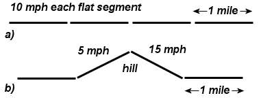
One rate example that I personally relate to contrasts riding a bike in flat versus hilly country. If I set a goal of traveling between points A and B in the shortest amount of time, I know from experience how the rates affect my progress. For one, I know that the hilly country would always result in the longest travel time. For the figure below, I set up an example of a x=4 mile course consisting of four 1-mile segments. On flat ground (a) I can cover the entire course in T=24 minutes if I maintain a constant speed of r=10 mph (T = x/r = 4/10*60).

For the hilly course (b), one segment becomes steep enough that the constant rate drops to 5 mph. Work out the example, and you will find that the time it takes to cover the course will exceed 24 minutes for any finite value of speed going down the backside of the hill. For a 15 mph downhill, the extra time amounts to 4 minutes. Only an infinite downhill speed will match the flat course in completion time. And that jives exactly with the agonizing learned behavior that comes with the physical experience.

Yet if we quickly glanced at the problem as stated we may incorrectly assume that the two hill rates average out to 10 = (5 +15)/2 and if not careful we may then incorrectly conclude that we could certainly go faster than 15 mph on the backside and actually complete the hilly course faster!

The mismatch between the obvious physical intuition we get from riding the bike course and the lack of intuition we get by looking at the abstract problem formulation extends to other domains.

This same trap exists for a rate of return investment strategy. The lifetime of an investment follows the same hilly trajectory, yet we don't experience the same visceral impact in our perception of how varying rates modify our expected rate of return. In other words, as a group of heuristically-driven humans, we have no sense of how and why we can't keep up a predictable rate of return. We also don't necessarily do a robustness analysis in our head to see how excursions in the rate will affect the result.

With that as a backdrop, let me formulate the investment problem and its set of premises. To start, assume the variation in our rate as very conservative in that we do not allow it to go negative, which would indicate that we eat away at the principal. Over the course of time, we have an idea of an average rate, r0, but we have no idea of how much it will vary around that value. So we use the Maximum Entropy Principle to provide us an unbiased distribution around r0, matching our uncertainty in the actual numbers.

p(r) = (1/r0) * exp(-r/r0)

This weights the rates toward lower values and r0 essentially indicates our expectation of future payouts. Over an ensemble of r values, the conditional probability of an initial investment matching the original principle in time t becomes:

P(t | r0) = exp (-1/(t*r0))

Treating the set as an ensemble versus treating a single case while varying r continuously will result in the same expression (addendum: see ref [2]). This has the correct boundary conditions: at t=0 we have no chance of getting an immediate return, and if we wait to t=infinity, we will definitely reach our investment goal (not considering the investment going belly-up).

This result, even though it takes but a couple of lines of derivation, has huge implications. As we really don't know the rate of return we eventually get dealt, it shouldn't really surprise us that at T=1/r0 the probability of achieving our expected rate of return is only P(t=T | r0) = exp (-1) = 0.367.

Yet this runs counter to some of our pre-conceived notions. If someone has convinced us that we would get our principal back in T=1/r0 years with a certainty closer to unity (1 not 0.367), this should open our eyes a little.
(never mind the fine print in the disclaimer, as nobody really explained that either)
It boils down to the uncertainty that we have in the rate, as to whether it will go through a hilly trajectory or a flat one, generates a huge bias in favor of a long hilly latency. We just don't find this intuitively obvious when it comes to volatile investments. We continue to ride the hills, while forever thinking we pedal on flat terrain.

But it gets worse than this. For one, r can go negative. That would certainly extend the time in meeting our goal. But consider a more subtle question: What happens if we just wait another T=1/r0 years? Will we get our principal back then?

According to the formula, reaching this goal becomes only slightly more likely.

P(t=2*T | r0) = exp (-1/2) = 0.606.

This continues on into fat-tail territory. Even after 10 cycles of T, we will only on average reach 0.9 or a 90% probability of matching our initial principal. The fat-tail becomes essentially a 1/t asymptotic climb to the expected return. This turns into a variation of the 90/10 heuristic whereby 10% of the investors absorb 90% of the hurt or 35% get 65% of the benefit. Not an overpowering rule, but small advantages can reap large rewards in any investment strategy.

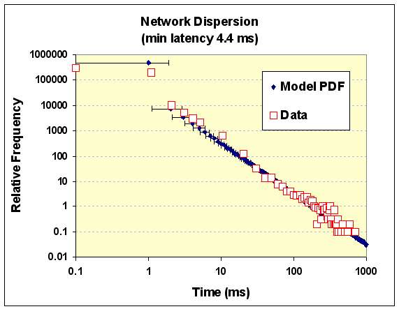
Although it will never happen due to the finite limits set forth, the expected time to reach the objective logarithmically diverges to infinity. This occurs due to the 1/t^2 decay present in the probability density function (the blue single-sided entroplet in the figure to the right). Although progressively rarer, the size of the delay compensates and pushes the expected value inexorably forward in time.

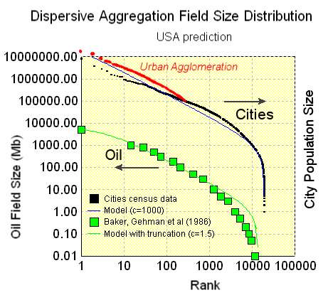
A related effect occurs in finding large oil reservoirs. We get lots of our oil from a few large reservoirs, while the investment monopoly money pays out from the fat-tail of low rate of return investments.

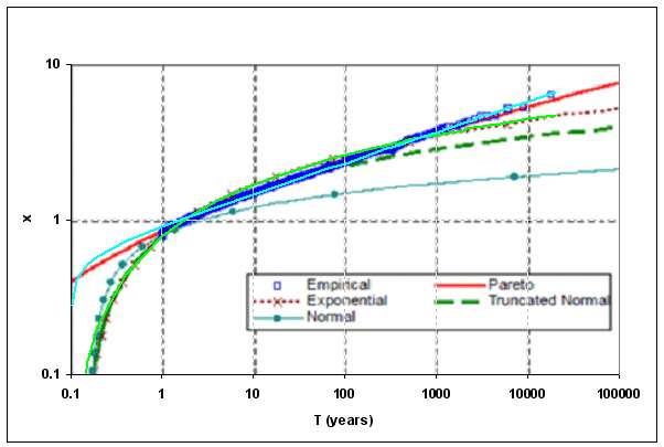
Now you can say that this really only shows the return for a hypothetical ensemble-averaged investor. We shouldn't preclude that individual investors can make money. But the individual does not concern me, as a larger filter predicts the prevailing Wall Street strategy perpetrated on the naive investor class, effectively operating under Maximum Entropy conditions. Unwittingly, the mass of investors get dragged into a Pareto Law wealth distribution, simply by making investments under a veil of uncertainty. In this situation, 37% of investors "beat the system", while 63% of the investors are losers in the sense that they don't make the expected payoff (see the adjacent figure). They contribute to the huge number of investors who only gain back a fraction of the return in the expected time. It seems reasonable that a split of 50/50 would at least place the returns in Las Vegas territory for predictability and fair play.

So who makes the money? Of course the middleman makes lots of money. So too does the insider who can reduce the uncertainty in p(r). And so do the investors who have fast computers who can track the rate changes quicker than others. The list of profiteers can go on.

The cold-footed investor who keeps changing his portfolio will turn out even worse-off. Each time that he misses the 37% cutoff, it makes it even more likely that he will miss it next time as well. (That happens in project scheduling as well where the fat-tails just get fatter) The definition of insanity is "doing the same thing over and over again and expecting different results".

Putting it charitably, the elite investment community either understands the concept as subliminal tacit knowledge or have gradually adapted to it as their lifeblood. In a conspiratorial bent, you can imagine they all know that this occurs and have done a great job of hiding it. I can't say for sure as I don't even know what to call this analysis, other than a simple robustness test.

The path forward. If you look at the results and feel that this idea may have some merit, I can offer up a few pieces of advice. Don't try to win at game theoretic problems. Someone else will always end up winning the game. In my view, try to place investments into guaranteed rate of return vehicles and work for your money. A volatile investment that takes 3 times as long to reach a goal than predicted might end up providing exactly the same return as a fixed return investment ot 1/3 the interest.

On a larger scale, we could forbid investment houses to ever mention or advertise average rates of return. Simply by changing the phrase to "average time to reach 100% return on investment", we could eliminate the fat-tails from the picture. See in the graph below how the time-based cumulative exponentially closes in on an asymptote, the very definition of a "thin tail". 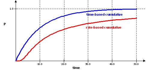Unfortunately, no one could reasonably estimate a good time number for most volatile investments, as that number would approach infinity according to maximum entropy on the rates. So no wonder we only see rates mentioned, or barring that an example of the growth of a historical investment set in today's hypothetical terms.

Briefly reflect back to the biking analogy. Take the case of a Tour de France bicycle stage through the Alps. You can estimate an average speed based on a sample, but the actual stage time for a larger sample will diverge based on the variability of rider's climbing rates. That becomes essentially the grueling game and bait/switch strategy that the investor class has placed us in. They have us thinking that we can finish the race in a timely fashion based on some unsubstantiated range in numbers. In sum, they realize the value of uncertainty.

So the only way to defeat fat-tails is to lobby to have better information available, but that works against the game theory strategies put in place by Wall Street.

So for this small window on investments, all that heavy duty quantitative analysis stuff goes out the window. It acts as a mere smokescreen for the back-room quants on Wall Street to use whatever they can to gain advantage on the mass of investors who get duped on the ensemble scale. Individual investors exist as just a bunch of gas molecules in the statistical mechanics container.

We have to watch these games diligently. The right wing of the Bush administration almost pulled off a coup when they tried to hijack social security by proposing to lock it into Wall Street investments. Based on rate of return arguments, they could have easily fooled people into believing that their rate of return didn't include the huge entropic error bars. Potentially half of the expected rate of return could have gotten sucked up into the machine.

The caveat. I have reservations in this analysis only insofar as no one else has offered it up (to the best of my knowledge). I admit that Maximum Entropy dispersion of rates generates a huge variance that we have to deal with (it definitely does not classify as Normal statistics). I puzzle why fat-tail authority and random process expert N.N. Taleb hasn't used something like this as an example in one of his probability books. I also find it worrisome that something as simple as an ordinary equity investments with strong volatility would show such strong fat-tail behavior. Everything else I had seen concerning fat-tails had only hand-wavy support.

Fat-tails work to our advantage when it comes to finding super-giant oil reservoirs, but they don't when it comes to sociopathetic game theory as winners do the zero-sum dance at the expense of the losers.

Or is this just evolution and adaptation taking place at a higher level than occurs for the planet's wildlife species? The winners and losers there follow the relative abundance distribution in a similar Pareto Law relationship. Each case derives completely from a basic application of the Maximum Entropy Principle. This does seem to support the assertion that the second law of thermodynamics has some general applicability.

Unfortunately, many mathematicians don't approve of this kind of analysis because the Maximum Entropy Principle invokes Bayesian rule and to a certain school of statisticians, Bayesian reasoning is not a formally proper approach. I suspect they would want me to start from a random walk premise and invoke a Levy flight or fractional Brownian motion. Yet it continues to explain puzzling behaviors over and over again from a practical point of view. See the Various Consequences blog for lots of interesting discussion concerning Jaynes' ideas on how to apply Bayesian and entropy to real problems.

I am making a big leap here as I barely touch the waters of financial trading or economics[1]. In general, game theory describes economic activity, and game theory problems are intractably difficult to solve. This may not actually constitute a real science, just psychological gamesmanship. I only worked this out to satisfy my own curiosity and would not feel bad if someone corrects me.

"In any field, the Establishment is seldom in pursuit of the truth, because it is composed of those who sincerely believe that they are already in possession of it.

-- E.T. Jaynes

---
[1] At one time I half-convinced myself that a ratchet effect took place due to the asymmetries of positive and negative stock market percentage increments. There is something odd about a 1% increase not precisely compensating a 1% decrease in the value of an investment. http://mobjectivist.blogspot.com/2006/05/taking-stock.html

[2] The rates can't swing wildly as in day-to-day market fluctuations or very fast volatility. The rates will average out normally in this case. Time has to play a factor. If the strength of an investment has a relation to the growth potential of a firm then the slow growth of a firm has to take place over a period of time. To use the hill-climbing analogy, a struggling company needs to spend extra time to climb a hill to meet its growth objectives since they have a lower effective speed. Other more capable firms can climb the hill faster so they do not spend a lot of time getting there. See a previous post discussing scheduling bottlenecks, where we can show how companies can struggle in putting product out the door, generating very fat tails. Companies that struggle spend a longer time in the trough, so to speak. Companies that don't spend less time. So the investor gets trapped in one or the other kinds of investments, leading to a slower volatility trap.
If equity investments do not relate to the firm's long-term growth potential then we see nothing more than gaming strategies dealing with Monopoly money (i.e. pure game theory). Market rates go up and down on a whim or on the current days speculation and you can lose money off of deviations from the average only if compounding growth takes place: see volatility drag or risk drag. The fact that more people have awareness of volatility drag indicates perhaps that investors practice more speculative analysis than have concern over the "market fundamentals". No wonder we get surprised by fat-tails, as those demonstrate the real risk in investments and the frequency of slow growth.