Understanding Recovery Factors

A recent TOD post on reserve growth by Rembrandt Kopelaar motivated this analysis.

The recovery factor indicates how much oil that one can recover from the original estimate. This has important implications for the the ultimately recovery resources, and increases in recovery rate has implications for reserve growth.

First of all, we should acknowledge that we still have uncertainty as to the amount of original oil in place, so that the recovery factor has two factors of uncertainty.

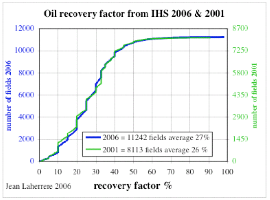
The cumulative distribution of reservoir recovery factor typically looks like the following S-shaped curve. The fastest upslope indicates the region closest to the average recovery factor.

Figure 1: Recovery Factor cumulative distribution function (from)

To understand the spread in the recovery factors, one has to first realize that all reservoirs have different characteristics. Some are more difficult to extract from and others have easier recovery factors. One of the principle first-order effects has to do with the size of the reservoir: bigger reservoirs typically have better recovery factors and as one reservoir engineer mentioned on TOD

"Reserve growth tends to happen in bigger fields because thats where you get the most bang for your buck"

So if we make the simple assumption that cumulative recovery factors (RF) have Maximum Entropy uncertainty or dispersion for a given Size:

P(RF) = 1-exp (-k*RF/Size)

this makes sense as the recovery factor will extend for larger fields.

Add to the mix that reservoir Sizes go approximately as (see here):

Pr(Size)= 1/(1+Median/Size)

Then a simple reduction in these sets of equations (with the key insight that RF ranges between 0 and 1, i.e. between 0 and 100%) gives us

P(RF) = 1 - exp(-k*RF*RF/(1-RF)/Median)

the ratio Median/k indicates the fractional average recovery factor relative to the median field size.

A set of curves for various k/Median values below:

Figure 2: Recovery Factor distribution functions assuming maximum entropy

Rembrandt provided some recovery factor curves originally supplied by Laherrere, and I fit these to the Median/k fractions below.

Figure 3: Recovery factor curves from Rembrandt's TOD post,
alongside the recovery factor model described here.

Laherrere also provided curves for natural gas, where recovery factors turn out much higher.

Figure 4: Recovery Factor distribution functions for natural gas.
Note that the recovery factor is much higher than for oil.
(Note: I had to fix the typo in the graph x-axis naming)

It looks like this derivation has strong universality underlying it. This remains a very simple and parsimonious model as it has only one sliding parameter. The parameter Median/k works in a scale-free fashion because both numerator and denominator have dimensions of size. This means that one can't muck with it that much -- as recovery factors increase, the underlying uncertainty will remain and the curves in Figure 2 will simply slide to the right over time while adjusting their shape. This will essentially describe the future reserve growth we can expect; the uncertainty in the underlying recovery factors will remain and thus we should see the limitations in the smearing of the cumulative distributions.

To reverse the entropic dispersion of nature and thus to overcome the recovery factor inefficiency, we will certainly have to expend extra energy.