M O B J E C T I V I S T: December 2007

The same dispersion that fits into the dispersive discovery model and reserve growth gives the climate change deniers a different type of fits.

I looked at Wharf Rat's analysis and it features some relatively straightforward assumptions.

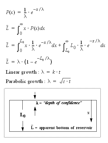
In general I think the standard premise of "dispersion" of time constants in climate change has the same validity on oil depletion analysis. Not only does dispersion play an effect on discovery profiles and reserve growth, but it also plays a key role in the log-normal distribution of reservoir sizes¹. For climate change, remember that not one single time constant rules over the temperature time series that the data analysts pour over. Interestingly, the dispersion has positive effects on oil resources, in that it leads to greater reserves than we may currently believe, but the same effect has negative consequence as the longer time scales in GW analysis lead to lags in heating that deniers such as Steven Schwartz evidently miss completely, and non-skeptical sorts like jrwakefield (a troll commenter on TOD) gobble up.

The deniers don't understand the math and it gives them fits.

¹ The USGS analysts that did the following study on crystal growth mechanisms may or may not know that their analysis has a strong analogy to reservoir growth. Millions of years ago, the dispersion in growth rates of primordial reservoirs caused the log-normal distribution of discovery sizes we see today. The math shakes out rather straightforwardly and I will try to show a derivation in the near future.

The evolution of the shape of a crystal size distribution (CSD) can be used to infer growth laws for crystals. For example, the often assumed constant growth rate law (dX/dt=k, where X is crystal diameter, t is time, and k is a constant) is unrealistic in most systems because it causes the variance of the CSD to approach 0 during growth, and because it destroys the shape of commonly occurring lognormal CSDs. Conversely, proportionate growth models (dX/dt=kX) best describe the evolution of CSDs in most systems. This law can be derived from a modified version of the Law of Proportionate Effect (LPE: X(j+1)=X(j) + v(j)e(j)X(j), where j refers to the growth cycle or time interval, v is a function of the proportion of the total volume of material available for each crystal for each growth cycle, and e is a random number that varies between 0 and 1). When v is large with respect to X, as is the case immediately after nucleation, the variance of the CSD increases with mean diameter and a lognormal CSD results. However, as X grows larger with respect to v, the variance remains constant as the mean crystal diameter increases, and the proportionate growth law is approximated. Simulating crystal growth by LPE using the Galoper computer program leads to some surprising conclusions, several of which have been confirmed by experiment: (1) If a small crystal doubles in diameter, a large crystal in the same system also will tend to double in diameter during the same time interval, even though such growth involves adding much more volume to the larger crystal; (2) Crystal growth has a random component (e), which indicates that one can not predict accurately the growth rate for individual crystals, but only for the distribution of crystals. This inherent randomness also accounts for crystal growth dispersion; (3) The relative shape of a CSD generally is determined soon after nucleation, and then is maintained during proportionate growth; (4) Crystal growth appears to occur in nanometer-size jumps, rather than continuously with time; and, (5) Proportionate growth occurs when reactants are supplied to the crystal surface by advection under stirred conditions, whereas constant growth is favored when supply is by diffusion under stagnant conditions.

I assert that we can explain the enigma of reserve growth of oil reservoirs by some simple physical considerations together with the dispersive formulation of growth rates.

Most of the observed growth seems to follow a "parabolic"¹ growth law that intuitively follows from the mathematics behind diffusion. The characteristic solution to diffusive growth as described by Fick's law shows an increase proportional to the square-root of time. Considering that one could model an arbitrary reservoir with a semi-permeable membrane that increases thickness with time, to first-order any concentration gradient across the thickness would show the characteristic square-root growth dependence.

However, we know that this growth law cannot sustain itself. We live in a finite universe, but the boundary conditions of Fick's law assume an infinite supply to draw from, leading to a theoretically infinite growth. And contrary to the perpetualist notion of an infinite supply of oil, we know that we should apply some type of boundary condition to reserve growth. But how do we do that?

A couple of years ago I tried computing a numerical solution to a self-limiting parabolic growth law. This seemed to fit the data effectively (see the figure above), but it seemed to veer toward Occam's territory a bit too much. A better, and more statistically and physically pleasing approach would include some considerations of the dimensionality of the reservoir volume and a maximum entropy spread in possible values for diffusive growth.

These actually fits the bill for a variation of dispersive growth with boundary conditions. By replacing a power-law growth rate in the original dispersive discovery model with a fractional (i.e. square-root) rate, we obtain the same "parabolic" growth curve initially -- but it also hits an asymptote related to the fixed volume defined by the L₀ parameter. Note the parabolic term in the growth law in the figure below.

The set of curves for various growth laws (both fractional power and integral power) looks like the following:

I can't tell whether the data values match the fractional power-law of 0.5 (square-root) or 0.6 better, but the general trend demonstrates itself effectively.

The green curve shows the 0.6 power-law, and both 0.5 and 0.6 curves reach an asymptote of 15. The asymptotic value obviously stays below infinity but it also approaches a value higher than the self-limiting numerical solution (see also that USGS's Attanasi and Root have extrapolated to a value near this but give no asymptote).

Khebab from TOD and Graphoilogy has incorporated some of the Arrington,Verma reserve growth models to extrapolate the shock model and its hybrid variant to enable predictive forecasts. This model may help that particular analysis because of its finite asymptote and closed form solution.

I can imagine that this model should also have some applicability to the analysis of creaming curves, where the important goal remains to identify the asymptote. Peak oil contrarians such as Michael Lynch continue to have a field day in criticizing creeping increases in creaming curves -- without a good model, I can imagine he has a point. Until now.

¹A bit of a misnomer, "parabolic" refers to the growth in time with thickness, not thickness with time, which would lead to proportional square-root growth. Blame Andy Grove of Intel.