Dispersive Diffusion model of Reserve Growth

I assert that we can explain the enigma of reserve growth of oil reservoirs by some simple physical considerations together with the dispersive formulation of growth rates.

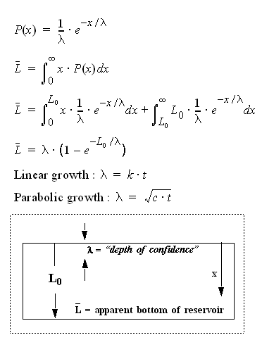
Most of the observed growth seems to follow a "parabolic"¹ growth law that intuitively follows from the mathematics behind diffusion. The characteristic solution to diffusive growth as described by Fick's law shows an increase proportional to the square-root of time. Considering that one could model an arbitrary reservoir with a semi-permeable membrane that increases thickness with time, to first-order any concentration gradient across the thickness would show the characteristic square-root growth dependence.

However, we know that this growth law cannot sustain itself. We live in a finite universe, but the boundary conditions of Fick's law assume an infinite supply to draw from, leading to a theoretically infinite growth. And contrary to the perpetualist notion of an infinite supply of oil, we know that we should apply some type of boundary condition to reserve growth. But how do we do that?

A couple of years ago I tried computing a numerical solution to a self-limiting parabolic growth law. This seemed to fit the data effectively (see the figure above), but it seemed to veer toward Occam's territory a bit too much. A better, and more statistically and physically pleasing approach would include some considerations of the dimensionality of the reservoir volume and a maximum entropy spread in possible values for diffusive growth.

These actually fits the bill for a variation of dispersive growth with boundary conditions. By replacing a power-law growth rate in the original dispersive discovery model with a fractional (i.e. square-root) rate, we obtain the same "parabolic" growth curve initially -- but it also hits an asymptote related to the fixed volume defined by the L₀ parameter. Note the parabolic term in the growth law in the figure below.


The set of curves for various growth laws (both fractional power and integral power) looks like the following:


I can't tell whether the data values match the fractional power-law of 0.5 (square-root) or 0.6 better, but the general trend demonstrates itself effectively.

The green curve shows the 0.6 power-law, and both 0.5 and 0.6 curves reach an asymptote of 15. The asymptotic value obviously stays below infinity but it also approaches a value higher than the self-limiting numerical solution (see also that USGS's Attanasi and Root have extrapolated to a value near this but give no asymptote).

Khebab from TOD and Graphoilogy has incorporated some of the Arrington,Verma reserve growth models to extrapolate the shock model and its hybrid variant to enable predictive forecasts. This model may help that particular analysis because of its finite asymptote and closed form solution.

I can imagine that this model should also have some applicability to the analysis of creaming curves, where the important goal remains to identify the asymptote. Peak oil contrarians such as Michael Lynch continue to have a field day in criticizing creeping increases in creaming curves -- without a good model, I can imagine he has a point. Until now.

---

¹A bit of a misnomer, "parabolic" refers to the growth in time with thickness, not thickness with time, which would lead to proportional square-root growth. Blame Andy Grove of Intel.