Observation of Shocklets in Action

I coined the term shocklet here to describe the statistically averaged production response to an oil discovery. This building block kernel allows one to deconstruct the macroscopic aggregation of all production responses into a representative sample for a single field. In other words, it essentially works backwards from the macroscopic to an equivalent expected value picture of the isolated microscopic case. As an analogy, it serves the same purpose of quantifying the expected miles traveled for the average person per day from the cumulative miles traveled for everyone in a larger population.

In that respect the shocklet formulation adds nothing fundamentally new to the Dispersive Discovery (DD)/Oil Shock model foundation, but does provide extra insight and perspective, and perhaps some flexibility into how and where to apply the model. And anything to unify with what Khebab has investigated, ala loglets, can't hurt.

Khebab pointed me to this article by B.Michel and noticed a resemblance to the basic shocklet curve:
Oil Production: A probabilistic model of the Hubbert curve

I did see this paper earlier in relation to the shocklet post and the referenced Stark/Bentley entry at TOD. Stark had basically taken a triangular heuristic as a kernel function to explain Dudley's simple model and made mention of the Michel paper to relate the two. Stark essentially rediscovered the idea of convolution without labeling it as such. I made notice of this at the time:

[-] WebHubbleTelescope on August 7, 2008 - 6:12pm

Khebab, I always think of the simplest explanation for a 2nd order Gamma is an exponential damped maturation/reserve growth fuction convolved with a expontial damped extraction function, ala the oil shock model.

[-] Nate Hagens on August 7, 2008 - 6:48pm
I tend to agree. This will likely be the topic of our next TOD press release.

[-] Euan Mearns on August 8, 2008 - 2:59am
If we're gonna do a press release I'd like to check the math before it goes out.

[-] Nate Hagens on August 8, 2008 - 4:37pm
Deal. As long as I check the spelling.

[-] Khebab on August 7, 2008 - 8:51pm
I agree, it's an elegant and concise solution which has many interpretations.

Michel went a bit further and although had some insightful things to say, I thought he took a wrong and misguided path by focusing on distribution of field sizes. In general, certain sections of the paper seemed to exist in an incorrectly premised mirror universe of what I view as the valid model. I will get to that in a moment. More importantly, Khebab reminded me that Michel did generate very useful data reductions from the North Sea numbers. In particular, Figure 14 in Michel's paper contained a spline fit to the aggregate of all the individual production curves, normalized to fit the production peak rate and field size (i.e. final cumulative production) into an empirically established kernel function. The red curve below traces the spline fit generated by Michel.

The green curve represents the shocklet assuming a "seam" dispersive discovery profile convolved with a characteristic damped exponential extraction rate. As one of the key features of the shocklet curve, the initial convex upward cusp indicates an average transient delay in hitting the seam depth. You can also see this in the following figure below; in which I scanned and digitized the data from Michel's chart and ran a naive histogram averager on the results. Unfortunately, the clump of data points near the origin did not get sufficient weighting, and so the upward inflecting cusp doesn't look as strong as it should (but more so than the moving average spline indicates, which is a drawback of the spline method). The histogram also clearly shows the noisy parts of the curve, which occur predominantly in the tail.

I believe this provides an important substantiation of the DD shocklet kernel. The values for the two shocklet model parameters consist of the average time it takes to reach a seam depth and the average proportional extraction rate. Extrapolating from the normalized curve and using the scaling from Michel's figure 13, these give a value of 3.4 years for the seam DD characteristic time and 2 years for the extraction rate time constant (I assumed that Michel's Tau variable scales as approximately 20 years to one dimensionless unit according to Fig.13). Note that the extraction rate of 50%/year looks much steeper than the depletion rate of between 10% and 20% quoted elsewhere because the convolution of of dispersive discovery reserve growth does not compensate for the pure extraction rate; i.e. depletion rate does not equal extraction rate. As an aside, until we collectively understand this distinction we run the risk of misinterpreting how fast resources get depleted, much like someone who thinks that they have a good interest-bearing account without taking into account the compensating inflationary pressure on their savings.

The tail of the shocklet curve shows some interesting characteristics. As I said in an earlier post, the envelope of the family of DD curves tend to reach the same asymptote. For shocklets derived from DD, this tail goes as the reciprocal of first production time squared, 1/Time².

I also ran through the shocklet model through a Simulink/Matlab program, which has some practical benefit to those used to looking at a pure dataflow formulation of the model. A picture is supposedly worth a thousand words, so I won't spend any time explaining this :)

---

Turning back to Michel's paper, although I believe he did yeoman's work in his data reduction efforts, I don't agree with his mathematical premise at all. His rigorously formal proofs do not sway me either, since they stemmed from the same faulty initial assumptions.

1. Field Sizes. I contend that the distribution of field sizes generate only noise to the discovery profile (a second-order influence) . Michel bases his entire analysis on this field size factor and so misses the first order effects of the dispersive discovery factor. The North Sea in particular has a proclivity to of course favor the large and easy-to-get-to fields and therefore we should probably see those fields produced first and the smaller ones become shut-in earlier due to cost of operation. Yet we know that this does not happen in the general case; note the example of USA stripper wells that have very long lifetimes. So the assumption of an average proportional extraction rate across all discovery sizes remains a good approximation.
   
   
2. Gamma Distribution. This part gets really strange, because it comes tantalizing close to independently reinforcing the Oil Shock model. Michel describes the launching of production as a queuing problem where individual fields get stacked up as a set of stochastic latencies. As I understand it, each field gets serviced sequentially by its desirability. Then he makes the connection to a Gamma distribution much like the Oil Shock model does in certain situations. However, he blew the premise, because the fields don't get stacked up to first-order but the production process stages do; so you have to go through the fallow, construction, maturation, and extraction processes to match reality. Remember, greed rules over any orderly sequencing of fields put into play. The only place (besides an expensive region like the North Sea) that Michel's premise would work perhaps exists in some carefully rationed society -- but not in a free-market environment where profit and competition motivates the producers.

So connecting this to a URR, we go back to the field size argument. Michel can not place a cap on the ultimate recoveries from field size distribution alone, so ends up fitting more-or-less heuristically. If you base the cap on big fields alone, then a Black Swan event will completely subvert the scale of the curve. On the other hand, dispersive discovery accounts for this because it assumes a large searchable volume and follows the cumulative number of discoveries to establish an asymptote. Because of its conservative nature, a large Black Swan (i.e. improbable) discovery could occur in the future without statistically affecting the profile.

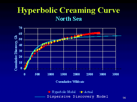
Besides, I would argue against Michel's maxRate/Size power-law as that convincing a tend. It looks like maxRate/Size shows about 0.1 for large fields and maybe 0.2 for fields 0.01x the size. The fact that the "big fields first" does not follow that strict a relationship would imply that the maxRate/Size works better by making it an invariant across the sizes. He really should have shown something like creaming curves with comparisons between "unsorted" and "sorted by size" to demonstrate the strength of that particular law. I suspect it will give second-order effects at best if the big/small variates are more randomized in time-order (especially in places other than the North Sea). The following curve from Jack Zagar and Colin Campbell shows a North Sea creaming curve. I have suggested before that cumulative # of wildcats tracks the dispersive discovery parameter of search depth or volume.


The blue curve superimposed shows the dispersive discovery model with a cumulative of approximately 60 GB (the red curve is a heuristic hyperbolic curve with no clear asymptotic limit). So how would this change if we add field size distribution to the dispersive discovery trend? I assert that it would only change the noise characteristics, whereas a true "large-field first" should make the initial slope much higher than shown. Now note that the authors Zagar and Campbell of the creaming curve repeated the conventional wisdom:

This so-called hyperbolic creaming curve is one of the more powerful tools. It plots cumulative oil discovery against cumulative wildcat exploration wells. This particular one is for the North Sea. The larger fields are found first; hence, the steeper slope at the beginning of the curve.

I emphasized a portion of the text to note that we do not have to explain the steeper slope by the so-called law of finding the largest fields first. The dispersive discovery model proves the antithesis to this conjecture as the shocklet and creaming curve fits to the data demonstrate. Most of the growth shown comes about simply from randomly trying to find a distribution of needles in a haystack. The size of the needles really makes no difference on how fast you find them.

I submit that it all comes down to which effect will become the first-order one. Judge on how well shocklets model the data and then try to disentangle the heuristics of Michel's model. I just hope that the analysis does not go down the field-size distribution path, as I fear that it will just contribute to that much more confusion in understanding the fundamental process involved in oil discovery and production.