Kernel of Logistic for Dispersive Discovery

The derivation of the dispersive discovery curve builds from a premise that individual discovery trajectories act on an ensemble of subvolumes within a larger volume (for example, the earth). Although the average rate of these arcs show an exponential acceleration over time, the individual rates get dispersed according to the Maximum Entropy Principle. The subvolumes also show an exponential PDF of sizes corresponding to the disorder expected in the geological search sizes of varying oil-bearing regions around the earth. Once the cumulative search in a subvolume completes, it reaches an asymptotic value proportional to the amount of oil in that region.

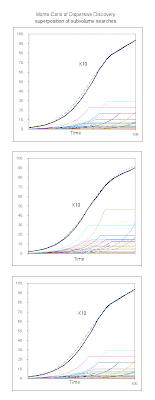
The following figure shows several Monte Carlo (MC) simulations of the build-up of the logistic Dispersive Discovery profile. This set of charts features only 100 sample traces accumulated per solid black line, yet the characteristic S-shape shows up clearly. The dashed curve behind the MC cumulative represents the logistic sigmoid function corresponding to theory.

In each of these cases, a gradual build-up of the individually colored profiles lead to nearly identical characteristic cumulative curves (save for counting noise).

I used a spreadsheet for this simulation as the MC algorithm reduces to a short algorithm. In the following formula, two exponential random variates sit in cells D$1 (growth dispersion) and D$2 (subvolume dispersion). An incremental time runs along column $A. The SIGN function truncates the individual cumulatives to truncate when the search reaches the subvolume limit. The term $A$1 represents the scaling term for the characteristic dispersion velocity spread. The last term acts like an integrator for $D$4 from the previous time step value D3.

+D$1*(SIGN(D$2-(D$1*$A4)/$A$1)+1)/2/$A$1+D3

If the time/$A series shows a linear growth in time, the summation of a series of these results in a hyperbolic asymptotic growth. If the time accelerates, we get the logistic form.

Each of the subvolume traces represent a discovery kernel function similar to a shocklet kernel. The physical realization of this becomes very intuitive, as prospecting for oil requires a complete survey of an entire subvolume, with the search accelerating over long periods of time as new technologies and tools become available. On the other hand, searches over very small regions may not have the aid of accelerated search and so the hyperbolic asymptotic growth results. This gives us the characteristic creaming curve in smaller basins. If you can understand when accelerating search applies and when linear search applies, it becomes very easy to predict what type of profile will occur in a region.

One thing I notice in the MC simulation is that the long term noise becomes greater as fewer discoveries contribute to the tail end of the curve. This may get reflected in the real statistics we will see as rather sparse fat-tail discoveries contribute to a long term decay.

A commenter at TOD recommended this visual as an aid to understanding how dispersion works.