Understanding Recovery Factors

A recent TOD post on reserve growth by Rembrandt Kopelaar motivated this analysis.

The recovery factor indicates how much oil that one can recover from the original estimate. This has important implications for the the ultimately recovery resources, and increases in recovery rate has implications for reserve growth.

First of all, we should acknowledge that we still have uncertainty as to the amount of original oil in place, so that the recovery factor has two factors of uncertainty.

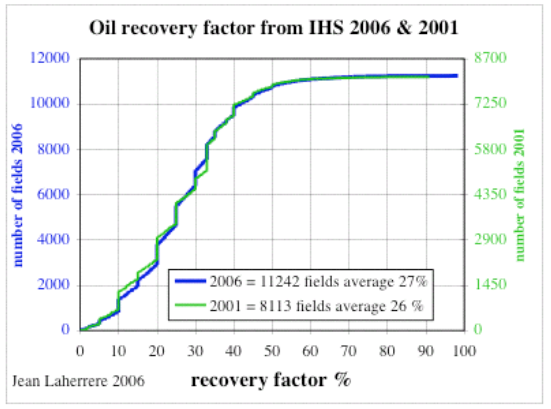
The cumulative distribution of reservoir recovery factor typically looks like the following S-shaped curve. The fastest upslope indicates the region closest to the average recovery factor.

Figure 1: Recovery Factor cumulative distribution function (from)

To understand the spread in the recovery factors, one has to first realize that all reservoirs have different characteristics. Some are more difficult to extract from and others have easier recovery factors. One of the principle first-order effects has to do with the size of the reservoir: bigger reservoirs typically have better recovery factors and as one reservoir engineer mentioned on TOD

"Reserve growth tends to happen in bigger fields because thats where you get the most bang for your buck"

So if we make the simple assumption that cumulative recovery factors (RF) have Maximum Entropy uncertainty or dispersion for a given Size:

P(RF) = 1-exp (-k*RF/Size)

this makes sense as the recovery factor will extend for larger fields.

Add to the mix that reservoir Sizes go approximately as (see here):

Pr(Size)= 1/(1+Median/Size)

Then a simple reduction in these sets of equations (with the key insight that RF ranges between 0 and 1, i.e. between 0 and 100%) gives us

P(RF) = 1 - exp(-k*RF*RF/(1-RF)/Median)

the ratio Median/k indicates the fractional average recovery factor relative to the median field size.

A set of curves for various k/Median values below:

Figure 2: Recovery Factor distribution functions assuming maximum entropy

Rembrandt provided some recovery factor curves originally supplied by Laherrere, and I fit these to the Median/k fractions below.

Figure 3: Recovery factor curves from Rembrandt's TOD post,
alongside the recovery factor model described here.

Laherrere also provided curves for natural gas, where recovery factors turn out much higher.

Figure 4: Recovery Factor distribution functions for natural gas.
Note that the recovery factor is much higher than for oil.
(Note: I had to fix the typo in the graph x-axis naming)

It looks like this derivation has strong universality underlying it. This remains a very simple and parsimonious model as it has only one sliding parameter. The parameter Median/k works in a scale-free fashion because both numerator and denominator have dimensions of size. This means that one can't muck with it that much -- as recovery factors increase, the underlying uncertainty will remain and the curves in Figure 2 will simply slide to the right over time while adjusting their shape. This will essentially describe the future reserve growth we can expect; the uncertainty in the underlying recovery factors will remain and thus we should see the limitations in the smearing of the cumulative distributions.

To reverse the entropic dispersion of nature and thus to overcome the recovery factor inefficiency, we will certainly have to expend extra energy.

Bird Surveys

This post either points out something pretty obvious or else it reveals something of practical benefit. You can judge for now.

I briefly made a reference to bird survey statistics when I wrote this post on econophysics and income modeling. I took a typical rank histogram of bird species abundance and fit it the best I could to a dispersive growth model, further described here. The generally observed trend follows that many species exist in the middle of abundance and relatively small numbers of species exist at each end of the spectrum -- few species exceedingly common (i.e. starling) and few species exceedingly rare (i.e. whooping crane). Since the bird data comes from a large area in North America, the best fit followed a meta-community growth model. The meta-community adjustment impacts the knee of the histogram curve and broadens the Preston plot, effectively smearing over geological ages that different species have had to adapt.

Figure 1: Preston plot (top) and
rank histogram (bottom) of relative bird species abundance

If we assume that the relative species abundance has a underlying model related to steady-state growth according to p(rate), where rate is the relative advantage for species reproduction and survival, then this should transitively might apply to disturbances to growth as well. Recently, I ran into a paper that actually tried to discern some universality in diverse growth papers, and it coincidentally used the bird survey data along with two economic measures of firm size and mutual fund size.

• Schwarzkopf, Yonathan, and J. Doyne Farmer, “The Cause of Universality in Growth Fluctuations.” Santa Fe Institute, (April 2010).
• Schwarzkopf, Yonathan, and J. Doyne Farmer. “Supporting Information — The Cause of Universality in Growth Fluctuations.” Santa Fe Institute.

I did the best I could with the figures in the paper but eventually went to the source, ftp://ftpext.usgs.gov/pub/er/md/laurel/BBS/DataFiles/, and used data from 1997 to 2009.

I applied the same abundance distribution as before and came up with the fit below (see blue and red curves below, data and model respectively). That provided a sanity check, but Schwarzkopf and Farmer indicated that the year-to-year relative growth fluctuations should also obey some fundamental behavior through the distribution of this metric:

RelativeGrowth(Year) = n(Year+1) / n(Year)

Sure enough, and for whatever reason, the "growth" in the surveyed data does show as much richness as the steady state averaged abundance distribution. The relative growth in terms of a fractional yearly change sits alongside the relative abundance curve below (in green). Notice right off the bat that the distribution of fractional changes drops off much more rapidly.

Figure 2 : The red meta-model curve smears the median from 200 to 60000

I believe that this has a simple explanation having to do with Poisson counting statistics. When estimating fractional yearly growth, we consider that the rarer bird species having the lowest abundance will contribute most strongly to fluctuation noise on year-to-year survey data. Values flipping from 1 to 2 will lead to 100% growth rates for example. (We have to ignore movements from 1 to 0 and 0 to 1 as these growths become infinite.

I devised a simple algorithm that takes two extreme values (R greater than 1 and R less than 1 ) and the steady state abundance N for each species. The lower bound of:

R1 = R * (1-sqrt(2/N))/(1+sqrt(2/N))

and the upper bound becomes:

R2 = R * (1+sqrt(2/N))/(1-sqrt(2/N))

The term 1.4/sqrt(N) derives from Poisson counting statistics in that the relative changes become inversely related to the size of the sample. We double count in this case because we don't know whether the direction will go up or down, relative to R, a number close to unity.

(This has much similarity to the model I just used in understanding language adoption. Small numbers of adopters experience suppressing fluctuations as 1/sqrt(N))

Expanding on the scale, the results of this algorithm are shown in Figure 3.

Figure 3 : Model of yearly growth fluctuation in terms of a cumulative distribution function

Placing it in terms of a binned probability density function, the results look like the following plot. Note the high counts match closely the data simply because the 1/sqrt(N) is relatively small. Away from these points, you can see the general trend develop even though the data is (understandably) obscured by the same counting noise.

Figure 4 : The probability density function of yearly growth fluctuations.

As an essential argument to take home, consider that a counting statistics argument probably accounts for the yearly growth fluctuations observed. Before you make any other assertions, you likely have to remove this source of noise. Looking at Figure 3 & 4, you can potentially see a slight bias toward positive growth for certain lower abundance species. This comes at the expense of lower decline elsewhere, except for some strong declines in several other low abundance species. This may indicate the natural ebb and flow of attrition and recovery in species populations, with some of these undergoing strong declines. I haven't done this but it makes sense to identify the species or sets of species associated with these fluctuations.

Two puzzling points also stick out. For one, I don't understand why Schwarzkopf and Farmer didn't immediately discern this effect. Their underlying rationale may have some of the same elements but it gets obscured by their complicated explanation. They do use a resampling technique (on 40+ years worth of data) but I didn't see much of a reference to conventional counting statistics, only the usual hand-wavy Levy flight arguments. They did find a power law of around-0.3 instead of the -0.5 we used for Poisson, so they may generate something equivalent to Poisson by drawing from a similar Levy distribution. Overall I find this violates Occam's razor, at least for this set of bird data .

Secondly, it seems that these differential growth curves have real significance in financial applications. More of the automated transactions look for short duration movements and I would think that ignoring counting statistics could lead the computers astray.

---

Epilogue

As an aside, when I first pulled the data off the USGS server, I didn't look closely at the data sets. It turns out that the years 1994,1995,1996 were included in the data but appeared to have much poorer sampling statistics. From 1994 to 1996, the samples got progressively larger but I didn't realize this when I first collected and processed the data.

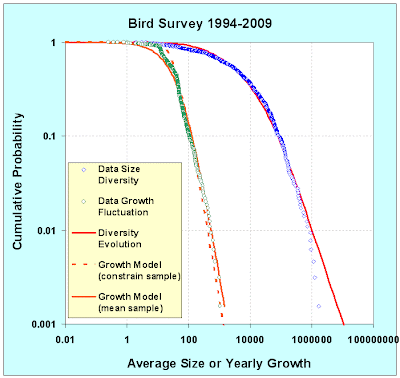
Figure 6 : CDF of larger data sample.
Note the strange hitch in the data growth fluctuation curve.

At the time, I figured that the slope had a simple explanation related to uncertainties in the surveying practice. I also saw some similarities to the uncertainties in stock market returns that I blogged about recently in an econophysics posting.

Say the survey delta time has a probability distribution with average time -- the T most likely related to the time between surveys:

pt(time) = (1/T)*exp(-time/T)

then we also assume that a surveyor tries to collect a certain amount of data, x, during the duration of the survey. We could characterize this as a mean, X, or some uniform interval. We don't have any knowledge of higher order moments to we just apply the Maximum Entropy Principle

px(x) = (1/X)*exp(-x/X)

The ratio between these two establishes the relative rate of growth, rate = X/T. We can derive the following cumulative quite easily:

P(rate) = T*rate/(T*rate +X)

The yearly growth rate fluctuations of course turn out as the second derivative of this function. We take one derivative to convert :

dp(rate)/drate = 2*T/X/(1+rate*T/X)^{^3}

On a cumulative plot as in Figure 6, this shows a power-law of order 2 (see the orange curve). Near the knee of the curve, it looks a bit sharper. If we use a uniform distribution of px(x) up to some maximum sample interval, then it matches the knee better (see the dashed curve).

So the simple theory says that much of the observed yearly fluctuation may arise simply due to sampling variations during the surveying interval. Plotting as a binned probability density function, the contrast shows up more clearly in Figure 7. In both cases is fit to X/T = 60. This number is bigger than unity because it looks like every year, the number of samples increases (I also did not divide by 15, the number of years in the survey).

But of course, the reason this maximum entropy model works as well as it does came about from real variation in the sampling techniques. Those years from 1994 to 1996 placed enough uncertainty and thus variance in the growth rates to completely smear the yearly growth fluctuation distribution.

Figure 7 : PDF of larger sample which had sampling variations.
Note that this has a much higher width than Figure 4.

Only in retrospect when I was trying to rationalize why a sampling variation this large would occur in a seemingly standardized yearly survey, did I find the real source of this variation. Clearly, the use of the Maximum Entropy Principle explains a lot, but you still may have to dig out the sources of the uncertainty.

Can we understand the statistics of something as straightforward as a bird survey? Probably, but as you can see, we have to go at it from a different angle than that typically recommended. I will keep an eye out if it has more widespread applicability; for now it obviously requires countable discrete entities.

Tower of Babel, How languages diversify

One pattern that has evaded linguists and cognitive scientists for some time relates to the quantitative distribution in human language diversity. Much like how plant and animal species diversify in a specific pattern, with very few species dominating within an ecosystem and relatively few species exceedingly rare, the same thing happens with natural languages. You find a few languages spoken by many people, and very few spoken seldomly,with the largest number occupying the middle.

Consider a simple model of language growth whereby adoption of languages occur over time by dispersion. The cumulative probability distribution for the number of languages is

P(n) = 1/(1+1/g(n))

This form derives from the application of the maximum entropy principle to any random variate where one only knows the mean in the growth rate and an assumed mean in the saturation level. I refer to this as entropic dispersion and have used this many applications before so I no longer feel a need to rederive this term every time I bring it up.

The key to applying entropic dispersion is in understanding the growth term g(n). In many cases n will grow linearly with time so the result will assume a hyperbolic shape. In another case, an exponential growth brought up by technology advances will result in a logistic sigmoid distribution. Neither of these likely explains the language adoption growth curve.

Intuitively one imagines that language adoption occurs in fits and starts. Initially a small group of people (at least two for arguments sake) have to convince other people on the utility of the language. But a natural fluctuation arises with small numbers as key proponents of the language will leave the picture and the growth of the language will only sustain itself when enough adopters come along and the law of large numbers starts to take hold. A real driving force to adoption doesn't exist, as ordinary people have no real clue as to what constitutes a "good" language, so that this random walk or Brownian motion has to play an important role in the early stages of adoption.

So with that as a premise, we have to determine how to model this effect mathematically. Incrementally we wish to show that the growth term gets suppressed by the potential for fluctuation in the early number of adopters. A weaker steady growth term will take over once a sufficiently large crowd joins the bandwagon.

dn = dt / (C/sqrt(n) + K)

In this differential formulation, you can see how the fluctuation term which goes as 1/sqrt(n) suppresses the initial growth until it reaches a steady state as the K term becomes more important. Integrating this term once and we get the implicit equation:

2*C*sqrt(n) + K*n = t

Plotting this for C=0.007 and K=0.000004, we get the following growth function.

Figure 1 : Growth function assuming suppression during early fluctuations

This makes a lot of sense as you can see that growth occurs very slowly until an accumulated time at which the linear term takes over. That becomes the saturation level for an expanding population base as the language has taken root.

To put this in stochastic terms assuming that the actual growth terms disperse across boundaries, we get the following cumulative dispersion (plugging the last equation into the first equation to simulate an ergodic steady state):

P(n) = 1/(1+1/g(n)) = 1/(1+1/(2*C*sqrt(n) + K*n))

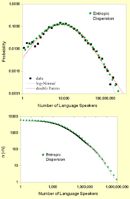
I took two sets of the distribution of population sizes of languages (DPL) of the Earth’s actually spoken languages from the references below and plotted the entropic dispersion alongside the data. The first reference provides the DPL in terms of a probability density function (i.e. the first derivative of P(n)) and the second as a cumulative distribution function. The values for C and K were as used above. The fit works parsimoniously well and it makes much more sense than the complicated explanations offered up previously for language distribution.

Figure 2 : Language diversity (top) probability density function (below) cumulative. The entropic dispersion model in green.

In summary, the two pieces to the puzzle are assuming dispersion according to the maximum entropy principle, and a suppressed growth rate due to fluctuations during the early adoption. This gives two power law slopes in the cumulative; 1/2 in the lower part of the curve and 1 in the higher part of the curve.

References

1. Scaling Relations for Diversity of Languages (2008)
2. Competition and fragmentation: a simple model generating
   lognormal-like distributions (2009)
3. Scaling laws of human interaction activity (2009)
   Discussions on the fluctuation term.
   

---

NY Math Teacher Howard A. Stern Uses Ingenuity To Overcome Failure Statistics

The public school teacher highlighted in the linked article has this to say:

"So much of math is about noticing patterns," says Stern, who should know. Before becoming a teacher, he was a finance analyst and a quality engineer.

I always try to seek interesting patterns in the data, but more to the point, I try to actually understand the behavior from a fundamental perspective.

One way Stern uses technology is by helping his students visualize his lessons through the use of graphing calculators.

Stern has it exactly right, if we treat knowledge seeking as a game, like a suduko puzzle, we can attract more people to science in general.

I think that the pattern in language distribution has similarities to that of innovation adoption as well, similar to what Rogers describes in his book "Diffusions of Innovations". I will try to look into this further as I think the dispersive arguments holds some promise as an analytical approach.

---

Stock Market as Econophysics Toy Problem

Consider a typical stock market. It consists of a number of stocks that show various rates of growth, R. Say that these have an average growth rate, r. Then by the Maximum Entropy Principle, the probability distribution function is:

pr(R) = 1/r*exp(-R/r)

We can solve this for an expected valuation, x, of some arbitrary stock after time, t.

n(x|t) = ∫ pr(R) δ(x-Rt) dR

This reduces to the marginal distribution:

n(x|t) = 1/(rt) * exp(-x/(rt))

In general, the growth of a stock only occurs over some average time, τ, which has its own Maximum Entropy probability distribution:

p(t) = 1/τ *exp(-t/τ)

So when the expected growth is averaged over expected times we get this integral:

n(x) = ∫ n(x|t) p(t) dt

We have almost solved our problem, but this integration reduces to an ugly transcendental function K₀ otherwise known as a modified Bessel function of the second kind and order 0.

n(x) = 2/(rτ) * K₀(2*sqrt(x/(rτ) ))

Fortunately, the K₀ function is available on any spreadsheet program (Excel, OpenOffice, etc) as the function BESSELK(X;0).

Let us try it out. I took 3500 stocks over the last decade (since 1999), and plotted the histogram of all rates of return below.


The red line is the Maximum Entropy model for the expected rate of return, n(x) where x is the rate of return. This has only a single adjustable parameter, the aggregate value rτ. We line this up with the peak which also happens to coincide with the mean return value. For the 10 year period, rτ = 2, essentially indicating an average doubling in the valuation of the average stock. This doesn't say anything about the stock market as a whole, which turned out pretty flat over the decade, only that certain high-rate-of-return stocks upped the average (much like the story of Bill Gates entering a room of average wage earners).

The following figure shows a Monte Carlo simulation where I draw 3500 samples from a rτ value of 1. This gives an idea of the amount of counting noise we might see.

I should point out that the MaxEnt model shows very little by way of excessively fat tails at high returns. A stock has to both survive a long time and grow at a rapid enough rate to get too far out in the tail. You see that in the data as only a couple of the stocks have returns greater than 100x. I don't rule out the possibility of high-return tails but we would need to put even more disorder in the pr(R) distribution than the MaxEnt provides for a mean return rate. The actual data seems a bit sharper and has more outliers than the Monte Carlo simulation, indicating some subtlety that I probably have missed. Yet, this demonstrates how to use the Maximum Entropy Principle most effectively -- you should only include the parameters that you can defend. From this minimal set of constraints you observe how far this can take you. In this case, I could only defend some concept of mean in rτ and then you get a distribution that reflects the uncertainty you have in the rest of the parameter space.

The stock market with its myriad of players follows an entropic model to first-order. All the agents seem to fill up the state space so that we can get a parsimonious fit to the data with an almost laughably simple econophysics model. For this model, the distribution curve on a log-log plot will always take on exactly that skewed shape (excepting for statistical noise of course) -- it will only shift laterally depending the general direction of the market.

The stock market becomes essentially a toy problem, no different than the explanation of statistical mechanics you may encounter in a physics course.

Has anyone else figured this out?

[EDIT]
Besides the slight fat-tail, which may be due to potential compounding growth similar to that found in individual incomes, the sharper peak may also have a second-order basis. This could result from a behavior called implied correlation which measures the synchronized behavior among stocks in the market. According to recent measurements, the correlation has hit all-time highs (the last around October 5). Qualitatively a high correlation would imply that the average growth rate r would show much less dispersion in that variate, and the dispersion would only apply to the length of time, t, that a stock rides the crest. Correlation essentially removes one of the parameters of variability from the model and the distribution sharpens up. The stock distribution then becomes the following simple damped exponential instead of the Bessel.

n(x) = 1/(rτ) * exp(-x/(rτ))

The figure below shows what happens when about 40% of the stocks would show this correlation (in green). The other 60% show independent variability or dispersion in the rates as per the original model.

I don't think this makes the collective stock behavior and more complex. I think it makes it simpler in fact. Implied correlation actually points to the future in the stock market. Dispersion in stock returns will narrow as all stocks move in unison. It makes it even more of a toy, with computers potentially dictating all movements.

Implied correlation has risen in the last few years (from here)

---

References
I personally don't deal with the stock market, preferring to watch it from afar. I found a few papers that try to understand this effect, but most just try to brute force fit it to various distributions.

1. Analysis of same data from Seeking Alpha
   
2. This paper is close but no cigar. It looks like they "detrend" the data to get of the skew, which I think misses the point :
   "Microscopic origin of non-Gaussian distributions of financial returns" (2007)
3. This book has info on the Bessel distribution:
   "Return distributions in finance", J. Knight and S. Satchell
4. Interesting from an econophysics perspective.
5. This book appears worthless:
   "Fat-Tailed and Skewed Asset Return Distributions", S.T. Rachev, F.J. Fabozzi, C Menn

Black-Scholes

Games for suits. This post has no relevance in the greater scheme of things.

As a premise, consider that the financial industry needs instruments of wealth creation that work opposite to that of stocks. For example, when stock prices remain low, then something else else should take up the slack -- otherwise important people won't make money. Wall Street invented derivatives, options, and other hedging methods to serve as an investment vehicle under these conditions.

We can try to show how this works.

If S is the stock price, then V ~ 1/S is an example "derivative" that works as a reciprocal to price. This becomes the normative description and defines the basic objective as to what the investment class wants to achieve -- an alternate form of income that balances swings in stock price, potentially reducing risk.

Further, we make the assumption that the derivative will grow or decline over time.

So we get:
V(S,t) = K/S * exp(a*t)

If a > 0 then the derivative will grow and if a is less than zero than the derivative will damp out over time. The term K is a constant of proportionality.

The infamous Black-Scholes equation supposedly governs the behaviour of derivatives with respect to stock prices (and time) according to this invariant:


The particulars may change but this formulation describes THE equation that Merton, Black, and Scholes devised to aid investors in making hedged investments using options and other derivatives. The way to read this equation is to note that derivatives will drift or diffuse into the space of the stock price, and proportional to the stock price itself. The drift term occurs due to the interest rate r providing a kind of forcing function. The derivative, V, can also grow due to pure interest rate compounding, as seen in the last term. Whether this actually holds or not, I don't really care as I don't participate in these schemes.

So if you look at it from a very neutral perspective you come up with some interesting observations. For one, you can trivially solve this partial differential equation for a generally disordered set of initial conditions. And the solution appears exactly the same as my first expression above:
V(S,t) = K/S * exp(a*t)

To verify this assertion, we test the expression in the B-S equation, substituting the partial derivatives as we go along.

a*K/S* exp(a*t) + 1/2(σS)²*2*K/S²*exp(a*t) - rS*K/S²*exp(a*t) - r*K/S * exp(a*t) = 0

Cancelling out all common factors:

a/S + 1/2(σS)²*2/S²- rS/S² - r/S = 0

Reducing the value of S

a/S + 1/2(σ)²*2/S- r/S - r/S = 0

a + 1/2(σ)²*2- r - r = 0

gets us to:

a = 2*r - σ²

The term r is proportional to interest, and σ is volatility or variance in stock price.

So this simple expression that I just cooked up will obey Black-Scholes as long as we choose the constant a term to correspond to the interest and volatility as shown above, and we get:
V(S,t) = K/S * exp((2*r - σ²)*t)

Note that if the volatility (i.e. diffusion) stays high relative to interest, the exponential will damp out with time. If interest (i.e. drift) goes higher than volatility, the exponential will accelerate, creating a huge amount of paper gains.

At this point someone will argue that this solution does not reflect reality. I beg to differ. When you make your bed of mathematical box-springs, you have to lie in it. This solution to Black-Scholes is perfectly fine as it gives a steady-state picture of the partial differential equation. The diffusional and drift components cancel with the right mix of production vs destruction in derivative wealth. If you don't like it, then come up with something different than that specific B-S equation.

I have a feeling that all the seeming complexity of financial quantitative analysis with its Ito calculus and Wiener processes acts as a shiny facade to a simple reality. The math exists to model the inverse relationship of stocks to derivatives. If this didn't happen -- and the lords of high finance absolutely require this relationship to make money -- the math as formulated would vanish from their toolbox. In other words, the math only exists to justify what the financial operatives want to see happen. Everyone appears to implicitly buy this mathematical artifice hook, line, and sinker.

Quantitative analysis and the "quants" who work it have created a fantasy land, where they do not want you to know how easily their quaint ornate universe reduces to a simple function. If they admitted to the charade, the mystery would all disappear and they would no longer have jobs.

Economics and finance does not constitute a science. In science you may need to use partial differential equations. For example, the Fokker-Planck equation shows up quite often -- which incidentally, the Black-Scholes equation shows some similarity to and the quant proponents of B-S certainly like to play up -- but it typically applies to real, physical systems where you use it to try to understand nature, not trying to model some artificial game-like behavior.

I can edit my solution into the Wikipedia page for Black-Scholes and I will bet that someone will immediately remove it. I harbor no illusions. The financial industry depends on the absence of real knowledge to achieve their objectives.

That explains why economics and finance do not classify as sciences; absolute truth does not matter to economists and financiers, only the art of deconstructing profit and the craft of phantom wealth creation does.

Please address editorial comments to: Postings, Main Incinerator, Department of Sanitation, North River Piers, New York, N.Y. 10019.

Lake Size Distributions

Our environment shows great diversity in the size and abundance in natural structures. Since we extract oil from our environment, it stands to reason that many of the same mechanisms leading to oil formation could also reveal themselves in more familiar natural phenomena. Take the size distribution of lakes as an example.

Freshwater lakes accumulate their volume in a manner analogous to the way that an underground reservoir accumulates oil. Over geologic time, water drifts into a basin at various rates and over a range in collecting regions. In the context of oil reservoirs, I have talked about this behavior before and the Maximum Entropy prediction of the size distribution leads to the following expression:

P(Size) = 1/(1+Median/Size)

Surveys of lake size show the same reciprocal power law dependence, with the exponent usually appearing arbitrarily close to one. In Figure 1 below, the data plotted on a ranked plot clearly shows this dependence over several orders of magnitude.

Figure 1: Northern Quebec lakes [1]

More revealing, in Figure 2 we can observe the bend in the curve that limits the number of small lakes in exact accordance to the equation. The agreement with such a simple model suggests that a universal behavior links the statistics between environmental phenomena as seemingly distinct as those of lakes and oil reservoirs.

Figure 2: Amazon lakes [2]

This provides other intuitive clues to how to think about reservoir sizing. Consider the fact that very few freshwater lakes reach gigantic portions, the Great Lakes serving as a prime example. Similarly, the rare occurrence of “super-giant” reservoirs follow from the same principles. We clearly won’t find any new huge freshwater lakes, while the future occurrence of super-giant oil reservoirs remains very doubtful just from the statistics of oil reservoirs found so far. Finding substantial numbers of super-giant reservoirs would result in deviations from the size distribution plot, making it very unlikely.

References
[1] K&C Science Report – Phase 1 Global Lake Census

[2] Estimation of the fractal dimension of terrain from Lake Size Distributions